Предисловие
Введение
Выборка отождествлений галактик из RFGC
- Этапы «очистки»
- Выбор единственного наилучшего отождествления
Подбор критериев отбора (g)
Подбор критериев отбора (r)
Подбор критериев отбора (i)
Подбор критериев отбора (z)
Подбор критериев отбора (y)
Отбор по выполнению критерия в любой полосе
- - Выводы
    - Таблица

Предисловие¶

Glossary¶

Term	Explanation
Term	Explanation
Detection	Catalog data for a single source from a single exposure.
Object	Catalog data for one or more associated detections.
OTA	Orthogonal Transfer Array. An OTA consists of an 8 x 8 array of 600 x 600 pixel CCD cells. The PS1 camera consists of 60 OTAs.
PSPS	Published Science Product System. This is the PS1 object database.
Sky cell	One tile in the PS1 tessellation of the sky.
Stack image	Image constructed by combining all useful warp images that overlap a single sky cell. Sometimes simply referred to as a "stack".
Stack detection	Catalog data for a single source from a stack image.
Stack object	Catalog data for one or more associated stack detections.
Tessellation	The scheme used to cover the spherical sky with a regular pattern of rectangular images in a manner that leaves no gaps in coverage.
Warp image	Image constructed by resampling a single exposure onto a canonical sky cell projection. Sometimes simply referred to as a "warp".
Ubercal	The process that uses comparisons in flux measurements from overlapping exposures to improve the global calibration.

Рабочие полосы¶

band	lambda	spec.res
g	481 nm	(R = 3.5)
r	617 nm	(R = 4.4)
i	752 nm	(R = 5.8)
z	866 nm	(R = 8.3)
y	962 nm	(R = 11.6)

Советы про использование звездных величин¶

Сравнение разных
- For point sources use PSF magnitudes.
  - Mean PSF magnitudes have the lowest noise (because the PSF model is most accurate in single-epoch images). They are good for brighter objects, but for objects near the single-epoch detection limit they will be biased (due to the absence of sub-threshold detections), and objects too faint to detect in a single epoch are missing.
  - Stack PSF magnitudes are noisier because the PSF model is less accurate. But the stack detections are more than a magnitude deeper and so have many more faint objects than mean detections.
  - Forced mean PSF magnitudes use PSF-fitting photometry on the single-epoch images at positions of stack detections. They are a reasonable compromise: they have slightly lower noise than the stack PSF magnitudes, and they are deep and unbiased (because they use data from all warps). Their noise is higher than the mean PSF magnitudes, however.
- For extended objects use Kron magnitudes.
  - Stack Kron magnitudes are usually the first choice as a general-purpose, deep magnitude.
  - de Vaucouleurs and exponential model fits could be better in some cases, and the mean measurements can be useful for objects that are barely resolved (where the PSF is important).
  - Extended object photometry using the PS1 catalog will require research and analysis by the user to determine the best approach.

Представляющие интерес параметры и таблицы¶

MeanObjectView = MeanObject JOIN ObjectThin -- фотометрия (PSF, Kron, апертурная) и координаты. Отсюда брали:
1. raMean, decMean
2. {filt}MeanKronMag

StackModelFitSer -- вписанный Серсик в изображение в разных полосах. Профиль Серсика у них такой (если убрать перекрестные члены): $$ \begin{aligned} \rho &= \sqrt{x^2/R_{xx}^2 + y^2/R_{yy}^2} \\ f &= I_0 e^{-\rho ^{1/n}} \end{aligned} $$ Отсюда брали:
1. {filt}SerRadius -- какой-то параметр профиля, скорее всего $R_{xx}$
2. {filt}SerAb --- отношение $b/a$ (а не $a/b$)
3. {filt}SerNu -- индекс $n$
4. {filt}SerPhi -- позиционный угол. Отсчитывается от направления на восток (почему-то)

ForcedGalaxyShape -- сюдя по всему, сначала изображение разбивается на 24 сектора, потом в каждом строится гистограмма, ищется медиана, и уже по этим точкам вписывается эллипс, но это неточно. Отсюда брали:
1. {filt}GalMajor -- большая полуось вписанного эллипса
2. {filt}GalMinor --- малая полуось вписанного эллипса
3. {filt}GalPhi -- позиционный угол. Отсчитывается от направления на восток (почему-то)

подробнее -- тут

Статьи¶

The Pan-STARRS1 Surveys, Chambers, K.C., et al.
Pan-STARRS Data Processing System, Magnier, E. A., et al.
Pan-STARRS Pixel Processing: Detrending, Warping, Stacking, Waters, C. Z., et al.
Pan-STARRS Pixel Analysis: Source Detection and Characterization, Magnier, E. A., et al.
Pan-STARRS Photometric and Astrometric Calibration, Magnier, E. A., et al.
The Pan-STARRS1 Database and Data Products, Flewelling, H. A., et al.

Про тонкости того, что означают те или иные параметры стоит идти в [4], но написано очень непонятно

Введение¶

Основная цель --- научиться выбирать плоские галактики в PanSTARRS. Судя по всему, они же будут видимыми с ребра, но для этого нужно анализировать вертикальный профиль, а такую задачу пока не пытались решать

Задачи:

Сопоставить какие-то объекты в PanSTARRS объектам из RFGC
Придумать критерий отбора плоских галактик, анализируя эти сопоставления
Протестировать эти критерии и отобрать кандидаты

Выборка отождествлений галактик из RFGC¶

Запрос чтобы достать все объекты в пределах заданного радиуса ($10''$) во всех полосах

WITH
nearobj AS (
    SELECT
        nb.objID, r.RFGC
    FROM
        MyDB.RFGCfull AS r
        CROSS APPLY fGetNearbyObjEq(r.RAJ2000, r.DEJ2000, 0.166) AS nb
    -- WHERE r.RFGC < 10
)
, panpos AS (
    SELECT
        o.objID, o.objName, o.raMean, o.decMean
    FROM
        MeanObjectView AS o
        INNER JOIN nearobj ON (o.objID=nearobj.objID)
)
, ser AS (
    SELECT s.*
    FROM
        StackModelFitSer AS s
        INNER JOIN nearobj ON (s.objID=nearobj.objID)
)
, seruniq AS (
    SELECT *
    FROM
    ( SELECT *
        ,ROW_NUMBER () OVER (
            PARTITION BY objID 
            ORDER BY bestDetection DESC, primaryDetection DESC
        ) AS rown -- enumerate inside common id group
        FROM ser
    ) AS t
    WHERE t.rown = 1 -- only first
)
, shape AS (
    SELECT s.*
    FROM ForcedGalaxyShape AS s
         INNER JOIN nearobj ON (s.objID=nearobj.objID)
)
, shapeuniq AS (
    SELECT *
    FROM ( 
        SELECT 
            *
          , ROW_NUMBER () OVER (
                PARTITION BY objID 
                ORDER BY
                CASE WHEN gGalFlags = 0 THEN 1
                     WHEN gGalFlags = 4 THEN 2
                     ELSE 3 END ASC,
                CASE WHEN rGalFlags = 0 THEN 1
                     WHEN rGalFlags = 4 THEN 2
                     ELSE 3 END ASC,
                CASE WHEN iGalFlags = 0 THEN 1
                     WHEN iGalFlags = 4 THEN 2
                     ELSE 3 END ASC,
                CASE WHEN zGalFlags = 0 THEN 1
                     WHEN zGalFlags = 4 THEN 2
                     ELSE 3 END ASC,
                CASE WHEN yGalFlags = 0 THEN 1
                     WHEN yGalFlags = 4 THEN 2
                     ELSE 3 END ASC
        ) AS rown -- enumerate inside common id group
        FROM shape
    ) AS t
    WHERE t.rown = 1 -- only first
)
, pet AS (
    SELECT p.*
    FROM
        StackPetrosian AS p
        INNER JOIN nearobj ON (p.objID=nearobj.objID)
)
, petuniq AS (
    SELECT *
    FROM
    ( SELECT *
        ,ROW_NUMBER () OVER (
            PARTITION BY objID 
            ORDER BY bestDetection DESC, primaryDetection DESC
        ) AS rown -- enumerate inside common id group
        FROM pet
    ) AS t
    WHERE t.rown = 1 -- only first
)
, kron AS (
    SELECT
        a.objID,
        a.bestDetection AS RadiusbestDetection, a.primaryDetection AS RadiusprimaryDetection,
        o.gMeanKronMag AS gkronMag, a.gKronRad AS gkronRadius,
        o.rMeanKronMag AS rkronMag, a.rKronRad AS rkronRadius,
        o.iMeanKronMag AS ikronMag, a.iKronRad AS ikronRadius,
        o.zMeanKronMag AS zkronMag, a.zKronRad AS zkronRadius,
        o.yMeanKronMag AS ykronMag, a.yKronRad AS ykronRadius
    FROM
        StackObjectAttributes AS a
        INNER JOIN nearobj ON (a.objID=nearobj.objID)
        LEFT JOIN MeanObjectView AS o on (o.objID=a.objID)
)
, kronuniq AS (
    SELECT *
    FROM
    ( SELECT *
        ,ROW_NUMBER () OVER (
            PARTITION BY objID 
            ORDER BY RadiusbestDetection DESC, RadiusprimaryDetection DESC
        ) AS rown -- enumerate inside common id group
        FROM kron
    ) AS t
    WHERE t.rown = 1 -- only first
)

SELECT 
    rfgc.*, 
    panpos.objID, 
    panpos.objName, 
    panpos.raMean, 
    panpos.decMean 
    ,
    seruniq.bestDetection AS serbestDetection,
    seruniq.primaryDetection AS serprimaryDetection
    ,
    seruniq.gSerRadius,seruniq.gSerAb,seruniq.gSerPhi,seruniq.gSerRa,seruniq.gSerDec,seruniq.gSerMag,
    seruniq.rSerRadius,seruniq.rSerAb,seruniq.rSerPhi,seruniq.rSerRa,seruniq.rSerDec,seruniq.rSerMag,
    seruniq.iSerRadius,seruniq.iSerAb,seruniq.iSerPhi,seruniq.iSerRa,seruniq.iSerDec,seruniq.iSerMag,
    seruniq.zSerRadius,seruniq.zSerAb,seruniq.zSerPhi,seruniq.zSerRa,seruniq.zSerDec,seruniq.zSerMag,
    seruniq.ySerRadius,seruniq.ySerAb,seruniq.ySerPhi,seruniq.ySerRa,seruniq.ySerDec,seruniq.ySerMag
    ,
    shapeuniq.gGalMinor,shapeuniq.gGalMajor,shapeuniq.gGalPhi,shapeuniq.gGalIndex,shapeuniq.gGalMag,shapeuniq.gGalFlags,
    shapeuniq.rGalMinor,shapeuniq.rGalMajor,shapeuniq.rGalPhi,shapeuniq.rGalIndex,shapeuniq.rGalMag,shapeuniq.rGalFlags,
    shapeuniq.iGalMinor,shapeuniq.iGalMajor,shapeuniq.iGalPhi,shapeuniq.iGalIndex,shapeuniq.iGalMag,shapeuniq.iGalFlags,
    shapeuniq.zGalMinor,shapeuniq.zGalMajor,shapeuniq.zGalPhi,shapeuniq.zGalIndex,shapeuniq.zGalMag,shapeuniq.zGalFlags,
    shapeuniq.yGalMinor,shapeuniq.yGalMajor,shapeuniq.yGalPhi,shapeuniq.yGalIndex,shapeuniq.yGalMag,shapeuniq.yGalFlags
    ,
    petuniq.bestDetection AS petbestDetection,
    petuniq.primaryDetection AS petprimaryDetection
    ,
    kronuniq.RadiusbestDetection AS kronRadiusbestDetection,
    kronuniq.RadiusprimaryDetection AS kronRadiusprimaryDetection
    , 
    petuniq.gpetMag,petuniq.gpetRadius,petuniq.rpetMag,petuniq.rpetRadius,petuniq.ipetMag,petuniq.ipetRadius,petuniq.zpetMag,petuniq.zpetRadius,petuniq.ypetMag,petuniq.ypetRadius, 
    kronuniq.gkronMag,kronuniq.gkronRadius,kronuniq.rkronMag,kronuniq.rkronRadius,kronuniq.ikronMag,kronuniq.ikronRadius,kronuniq.zkronMag,kronuniq.zkronRadius,kronuniq.ykronMag,kronuniq.ykronRadius 
INTO rfgc_nearby_multiband2

FROM MyDB.RFGCfull as rfgc
LEFT JOIN nearobj   ON nearobj.RFGC    = rfgc.RFGC
LEFT JOIN panpos    ON panpos.objID    = nearobj.objID
LEFT JOIN seruniq   ON seruniq.objID   = panpos.objID
LEFT JOIN shapeuniq ON shapeuniq.objID = seruniq.objID
LEFT JOIN kronuniq  ON kronuniq.objID  = shapeuniq.objID
LEFT JOIN petuniq   ON petuniq.objID   = kronuniq.objID

Здесь *uniq -- таблицы в которых выбрано «лучшее» детектирование для заданного objID

import numpy as np
import yaml
import numpy.ma as ma

from argparse import Namespace
import hashlib
import re

from IPython.display import display, HTML
from ipywidgets import interact, interactive, fixed, interact_manual
import ipywidgets as widgets

%load_ext autoreload
%autoreload 2

import matplotlib.pyplot as plt
from matplotlib import cm
from matplotlib.colors import SymLogNorm
import matplotlib as mpl

# строить картинки высокого разрешения
%matplotlib inline
%config InlineBackend.figure_format = 'retina'

import matplotlib.image as mpimg

from astropy.visualization import LogStretch, PercentileInterval

import plotly.graph_objects as go
import plotly.io as pio
import plotly.tools as plyt
import plotly.express as px
import plotly.figure_factory as ff
from plotly.subplots import make_subplots

png_renderer = pio.renderers["png"]
png_renderer.width = 800
png_renderer.height = 600
png_renderer.scale = 3

pio.renderers.default = "png"
pio.templates.default = "plotly_white"
#pio.renderers.default = 'png+jupyterlab'

from astropy.modeling import fitting, models
from astropy.coordinates import SkyCoord, Angle
import astropy.units as u

from joblib import Memory

cachedir = "./cached/"
memory = Memory(cachedir, verbose=0)

import pandas as pd

def mw_omit(l):
    b0 = 20  # deg
    rb = 15  # deg
    sigmab = 50  # deg
    lw = Angle(l, unit=u.deg).wrap_at('180d').value
    return b0 + rb*np.exp(-lw**2/(2*sigmab**2))

N = int(1e5)
points = np.random.uniform(-1, 1, size=(N, 3))
points = points[np.linalg.norm(points, axis=1) < 1]
coords = SkyCoord(points, representation_type='cartesian')

galaxies = pd.DataFrame({
    'ra'  : coords.cirs.ra,
    'dec' : coords.cirs.dec,
    'l'   : coords.galactic.l,
    'b'   : coords.galactic.b
})

galaxies_sel = galaxies[
    (np.abs(galaxies.b) > mw_omit(galaxies.l)) & 
    (galaxies.dec > -30)
]

gal_disc_ratio = len(galaxies_sel)/len(galaxies)

import seaborn as sb

# настройка стиля
sb.set(rc={'figure.figsize':(4,3)})
sb.set_style('whitegrid', {'grid.linestyle': ':'})
sb.set_palette("bright")

# ещё более тонкая настройка отображения картинок
dpi = 150
plt.rc('text', usetex=False)
plt.rc("savefig", dpi=dpi)
plt.rc("figure", dpi=dpi)
plt.rc('xtick', direction='in') 
plt.rc('ytick', direction='in')

SMALL_SIZE = 8
MEDIUM_SIZE = 10
BIGGER_SIZE = 12

plt.rc('font', size=SMALL_SIZE)          # controls default text sizes
plt.rc('axes', titlesize=SMALL_SIZE)     # fontsize of the axes title
plt.rc('axes', labelsize=MEDIUM_SIZE)    # fontsize of the x and y labels
plt.rc('xtick', labelsize=SMALL_SIZE)    # fontsize of the tick labels
plt.rc('ytick', labelsize=SMALL_SIZE)    # fontsize of the tick labels
plt.rc('legend', fontsize=SMALL_SIZE)    # legend fontsize
plt.rc('figure', titlesize=BIGGER_SIZE)  # fontsize of the figure title
#plt.rc('xtick.major', pad=5) 
#plt.rc('xtick.minor', pad=5)
#plt.rc('ytick.major', pad=5) 
#plt.rc('ytick.minor', pad=5)
plt.rc('lines', dotted_pattern = [0.5, 1.1])
plt.rc('axes', axisbelow=False)

from astropy.table import Table
from astropy.coordinates import Angle

import astropy.units as u

from astropy.io import fits
from astropy.wcs import WCS

from pathlib import Path

datapath = Path('data')
querypath = Path('queries')

name = f"rfgc_nearby_multiband2"
bands = 'grizy'
df = pd.read_hdf(datapath / (name + ".h5"))
#with pd.option_context("display.max_rows", 1000):
#    display(df[1:3].T)

for f in bands:
    df[f"{f}SerA"] = df[f"{f}SerRadius"]
    df[f"{f}SerB"] = df[f"{f}SerA"] * df[f"{f}SerAb"]
    df[f"{f}SerBa"] = 1/df[f"{f}SerAb"]
    
    df[f"{f}GalA"] = df[f"{f}GalMajor"] 
    df[f"{f}GalB"] = df[f"{f}GalMinor"] 
    df[f"{f}GalAb"] = df[f"{f}GalMinor"] / df[f"{f}GalMajor"]
    df[f"{f}GalBa"] = 1/df[f"{f}GalAb"]
    
df["AbO"] = df['bO'] / df['aO']

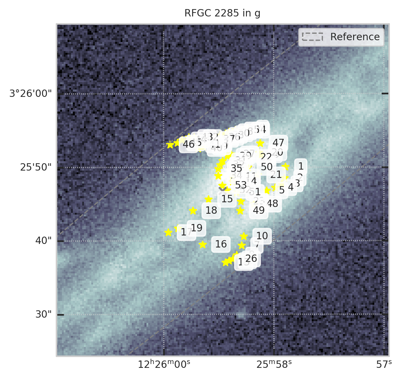
При таком выборе получается много отождествлений на один объект RFGC

ids_per_rfgc = df.groupby('RFGC').count()['objName']
ids_per_rfgc.sort_values(ascending=False)[0:10]

RFGC
2860    99
2212    96
769     87
2239    67
1190    67
4039    67
2449    61
1654    58
2162    56
286     54
Name: objName, dtype: int64

Например, для RFGC 2285 в полосе g

from code.crosstools import show_galaxy_rfgc

fig = plt.figure(figsize=(5,5))
subset = df[df.RFGC == 2285] 
show_galaxy_rfgc(subset.iloc[0], 'g', df=subset, image=True, fig=fig,
                 sersic=False, cleanp=False, kron=False, median=False, petrosian=False, exp=False, voculer=False,
                 zoom=4, transform=LogStretch(10) + PercentileInterval(99.5))

Этапы «очистки»¶

1. Выберем всё, что внутри эллипса, заданного RFGC и круга в $10'$ от положения центра в RFGC¶

from code.crosstools import inellipse

ra, dec = df['raMean'], df['decMean']
ra_ref, dec_ref = df['RAJ2000'], df['DEJ2000']

sigma_a = np.minimum(df['aO'], 10.)
sigma_b = np.minimum(df['bO'], 10.)

mask = inellipse((ra, dec), (ra_ref, dec_ref), -df['PA'], sigma_a, sigma_b)
matches_ref = df.loc[mask]

fig = plt.figure(figsize=(5,5))
t = matches_ref
subset = t[t.RFGC == 2285] 
show_galaxy_rfgc(subset.iloc[0], 'g', df=subset, image=True, fig=fig,
                 sersic=False, cleanp=False, kron=False, median=False, petrosian=False, exp=False, voculer=False,
                 zoom=4, transform=LogStretch(10) + PercentileInterval(99.5))

print(f"Осталось ~{len(t)/len(df)*100:.0f}% объектов")

Осталось ~64% объектов

2. Оставим только те, которые есть в `ForcedGalaxyShape` в заданной полосе¶

filt = 'g'

wshape = matches_ref.dropna(subset=[f"{filt}GalIndex"])

fig = plt.figure(figsize=(5,5))
t = wshape
subset = t[t.RFGC == 2285] 
show_galaxy_rfgc(subset.iloc[0], 'g', df=subset, image=True, fig=fig,
                 sersic=False, cleanp=False, kron=False, median=True, petrosian=False, exp=False, voculer=False,
                 zoom=4, transform=LogStretch(10) + PercentileInterval(99.5))

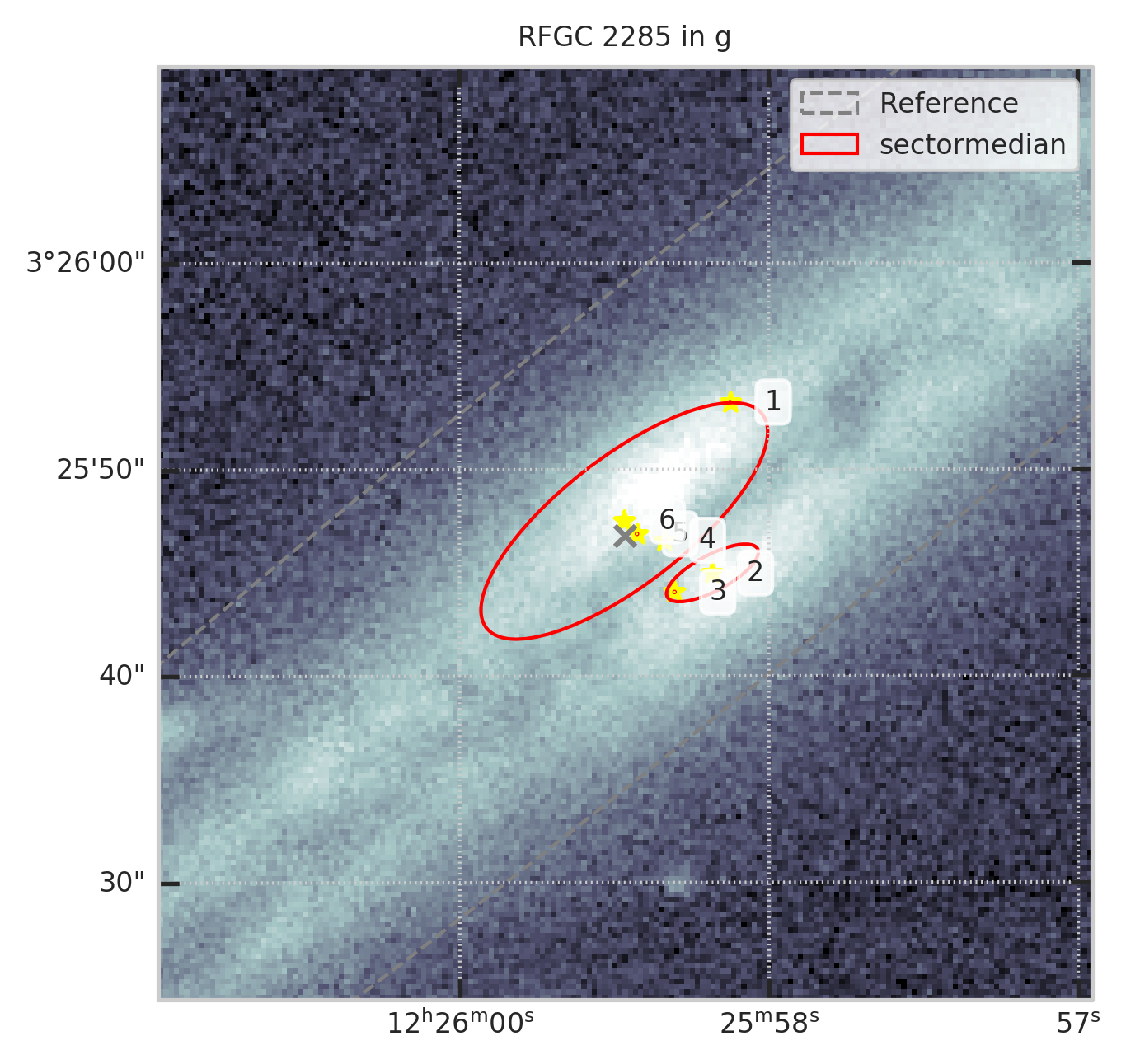
print(f"Осталось ~{len(t)/len(df)*100:.0f}% объектов")

Осталось ~6% объектов

ids_per_rfgc = t.groupby('RFGC').count()['objName']
ids_per_rfgc.sort_values(ascending=False)[0:10]

RFGC
2285    6
2015    5
3909    4
2860    4
677     4
982     4
4113    4
528     4
2132    3
2239    3
Name: objName, dtype: int64

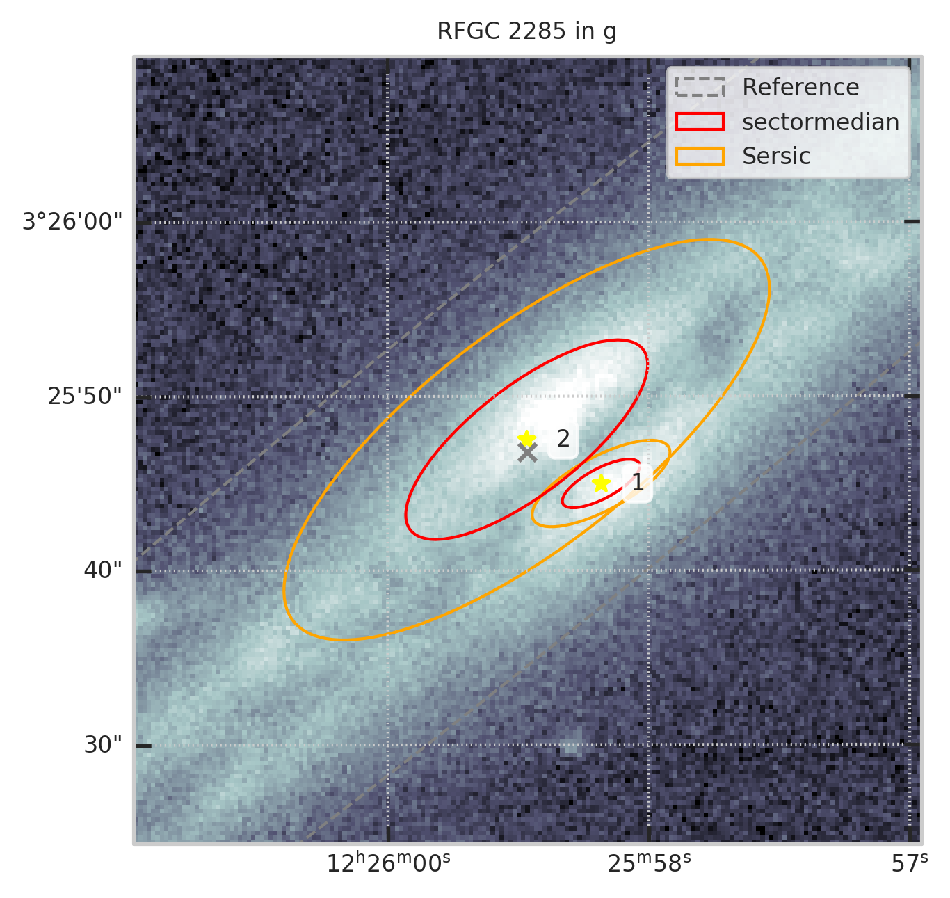
3. Оставим только те, для которых вписан Серсик в заданной полосе¶

filt = 'g'

fitted = wshape.dropna(subset=[f"{filt}SerRadius"])

fig = plt.figure(figsize=(5,5))
t = fitted
subset = t[t.RFGC == 2285] 
show_galaxy_rfgc(subset.iloc[0], 'g', df=subset, image=True, fig=fig,
                 sersic=True, cleanp=False, kron=False, median=True, petrosian=False, exp=False, voculer=False,
                 zoom=4, transform=LogStretch(10) + PercentileInterval(99.5))

print(f"Осталось ~{len(t)/len(df)*100:.1f}% объектов")

Осталось ~5.3% объектов

ids_per_rfgc = t.groupby('RFGC').count()['objName']
ids_per_rfgc.sort_values(ascending=False)[0:10]

RFGC
2285    6
982     4
677     4
2269    3
2442    3
396     3
1629    3
3909    3
4174    3
2556    3
Name: objName, dtype: int64

Все ещё остаются дубликаты

Посмотрим на объекты, которые PanSTARRS нашёл для галактики выше.

subset.loc[:, [f"{filt}SerRadius", f"{filt}SerAb", f"{filt}SerPhi", f"{filt}GalMajor", f"{filt}GalMinor", f"{filt}GalPhi"]]

Есть программный предел для радиуса Серсика: 0.05, позиционный угол и отношение осей при этом не определяются нормально

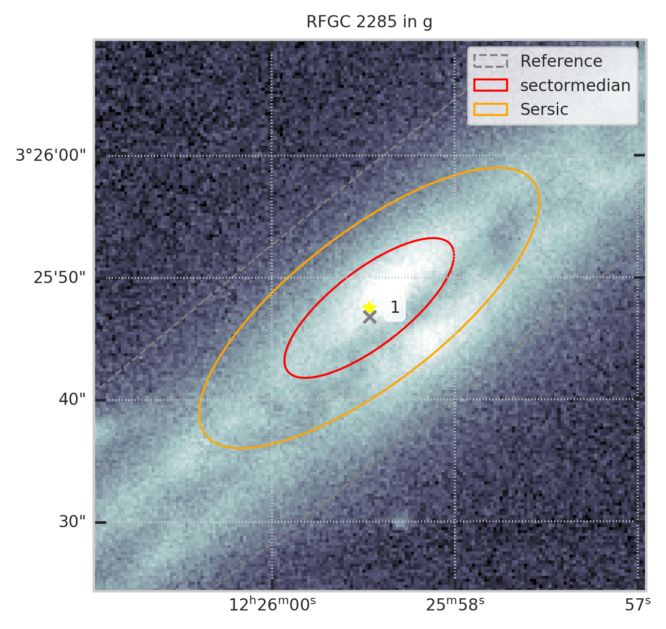
4. Отсеиваем программные ошибки вписания профиля¶

sane = fitted[fitted[f"{filt}SerA"] > 0.051]

fig = plt.figure(figsize=(5,5))
t = sane
subset = t[t.RFGC == 2285] 
show_galaxy_rfgc(subset.iloc[0], 'g', df=subset, image=True, fig=fig,
                 sersic=True, cleanp=False, kron=False, median=True, petrosian=False, exp=False, voculer=False,
                 zoom=4, transform=LogStretch(10) + PercentileInterval(99.5))

print(f"Осталось ~{len(t)/len(df)*100:.1f}% объектов")

Осталось ~5.2% объектов

ids_per_rfgc = t.groupby('RFGC').count()['objName']
ids_per_rfgc.sort_values(ascending=False)[0:10]

RFGC
982     4
677     4
4174    3
1267    3
2556    3
528     3
1922    3
2132    3
1325    3
188     3
Name: objName, dtype: int64

Часть мусора ушла, остались протяженные источники, но мало что потерялось

5. Выбор согласованных по позиционному углу источников¶

aligned = sane[(np.abs(sane[f"{filt}GalPhi"] - sane["PA"]) < 10) & 
               (np.abs(sane[f"{filt}SerPhi"] - sane["PA"]) < 10)]
#aligned.index= range(1, len(aligned)+1)

fig = plt.figure(figsize=(5,5))
t = aligned
subset = t[t.RFGC == 2285] 
show_galaxy_rfgc(subset.iloc[0], 'g', df=subset, image=True, fig=fig,
                 sersic=True, cleanp=False, kron=False, median=True, petrosian=False, exp=False, voculer=False,
                 zoom=4, transform=LogStretch(10) + PercentileInterval(99.5))

print(f"Осталось ~{len(t)/len(df)*100:.1f}% объектов")

Осталось ~4.8% объектов

ids_per_rfgc = t.groupby('RFGC').count()['objName']
ids_per_rfgc.sort_values(ascending=False)[0:10]

RFGC
1267    3
1603    3
396     3
4174    3
1922    2
1727    2
2568    2
273     2
1541    2
3840    2
Name: objName, dtype: int64

Выбор единственного наилучшего отождествления¶

Можно посмотреть, а в каких случаях объектов два

fig = plt.figure(figsize=(5,5))
t = aligned
subset = t[t.RFGC == 1922] 
show_galaxy_rfgc(subset.iloc[0], 'g', df=subset, image=True, fig=fig,
                 sersic=True, cleanp=False, kron=False, median=True, petrosian=False, exp=False, voculer=False,
                 zoom=1, transform=LogStretch(10) + PercentileInterval(99.5))

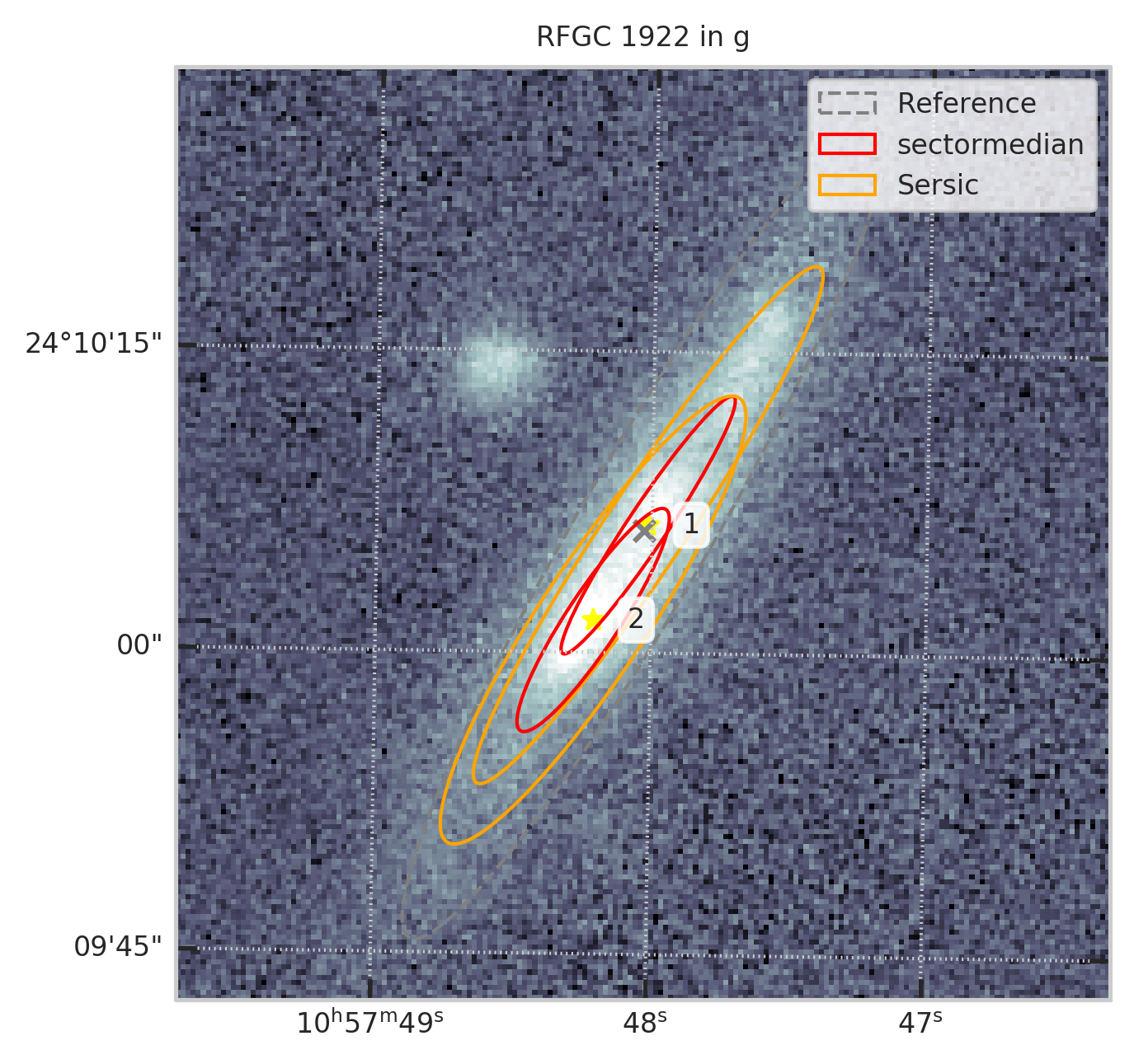
subset.loc[:, [f"{filt}SerRadius", f"{filt}SerAb", f"{filt}SerPhi", f"{filt}SerMag", 
               f"{filt}GalMajor", f"{filt}GalMinor", f"{filt}GalPhi", f"{filt}GalMag"]]

Какие есть варианты оставить по одному отождествлению на галактику RFGC:

Объект с наибольшей звездной величиной
Объект с наибольшей большой полуосью

В первом случае выше вероятность отождествить центр галактики, видимо так более осмысленно

biggestsersic_aligned = aligned.sort_values(["RFGC",f"{filt}SerA"],ascending=[True, False]).groupby('RFGC').head(1)
biggestsermag_aligned = aligned.sort_values(["RFGC",f"{filt}SerMag"],ascending=[True, True]).groupby('RFGC').head(1)

summary = {}
masks_t = {}
sqlconds = {}

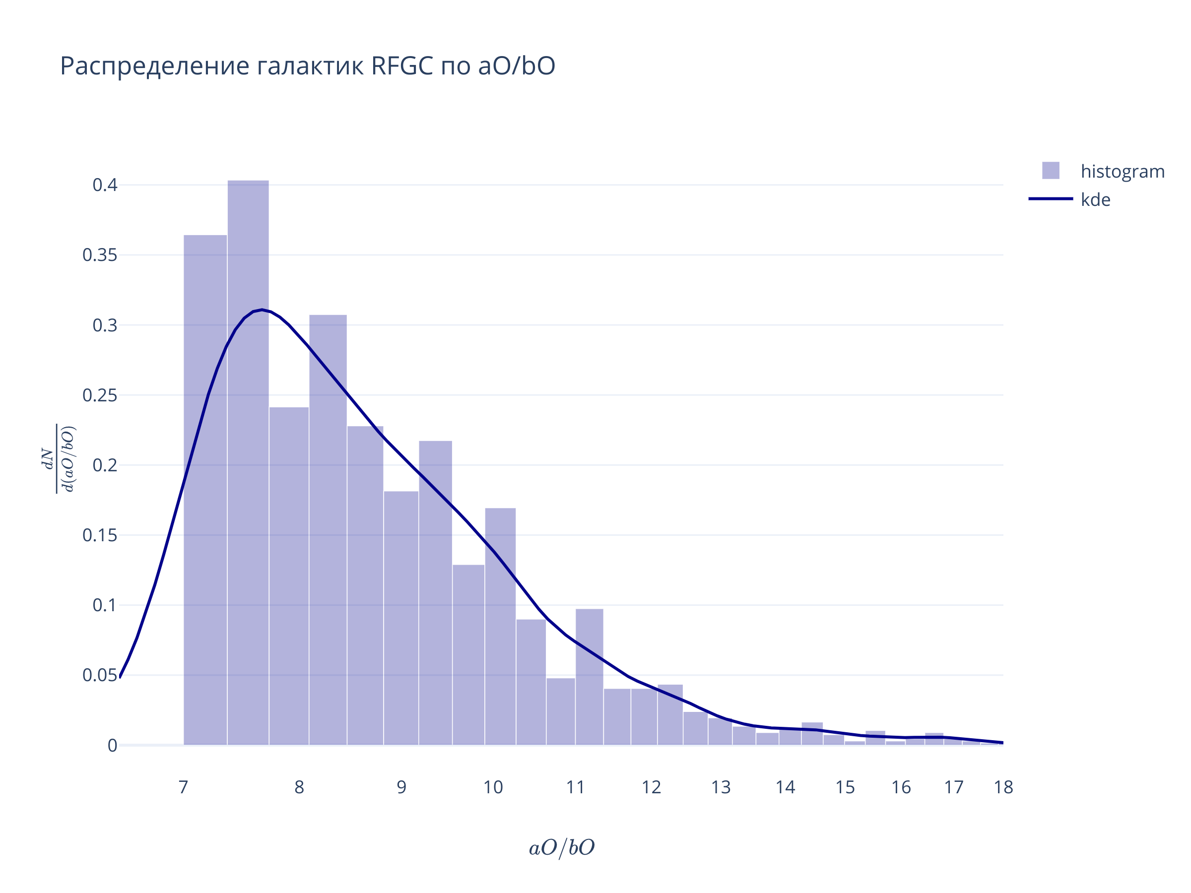
Подбор критериев отбора (g)¶

filt='g'

t = biggestsermag_aligned
t['BaO'] = 1/t['AbO']

from scipy.stats import gaussian_kde

yy, xx_e = np.histogram(t['BaO'], bins='auto', density=True)
xx = (xx_e[1:] + xx_e[:-1])/2

x1, x2 = np.log10(6.5), np.log10(18)
kernel = gaussian_kde(t['BaO'])
x_grid = np.logspace(x1, x2, 100)

fig = go.Figure(
    data = [
        go.Bar(x = xx, y = yy, width=xx[1]-xx[0], opacity=0.3, marker = {'color':'darkblue'}, name="histogram"),
        go.Scatter(x = x_grid, y = kernel(x_grid), line = {'color':'darkblue'}, name = 'kde')
    ],
    layout = go.Layout(xaxis = {'range':(x1, x2), 'type':'log', 'title':r"$aO/bO$"},
                       yaxis = {'title':r"$\frac{dN}{d (aO/bO)}$"},
                       title="Распределение галактик RFGC по aO/bO")
)
fig.show()

from code.plotutils import scatter_density_plotly
def scadensrfgc_ply(t, x, y, xrange, yrange, **kw):
    
    mask=(t[x]).between(*xrange) & (t[y].between(*yrange))
    rfgc_names = t.loc[mask, 'RFGC']

    xx = t.loc[mask, x]
    yy = t.loc[mask, y]

    mode = kw.pop('mode', 'kde')
    contours = kw.pop('contours', True)
    logx = kw.pop('logx', False)
    logy = kw.pop('logy', True)
    
    plots_kw = dict(mode=mode, modepars={'bins':(30,30)}, alpha=0.9,
                    pointlabels=rfgc_names, contours=contours, **kw)
    fig = scatter_density_plotly(xx, yy, xrange, yrange, x, y, logy=logy, logx=logx,
                           **plots_kw)
    return fig

fig = scadensrfgc_ply(
    biggestsermag_aligned, 
    'aO', 'BaO', 
    (17, 320), (6, 22),
    logx=True
)
fig.update_layout(autosize=False, width=600, height=500)
fig

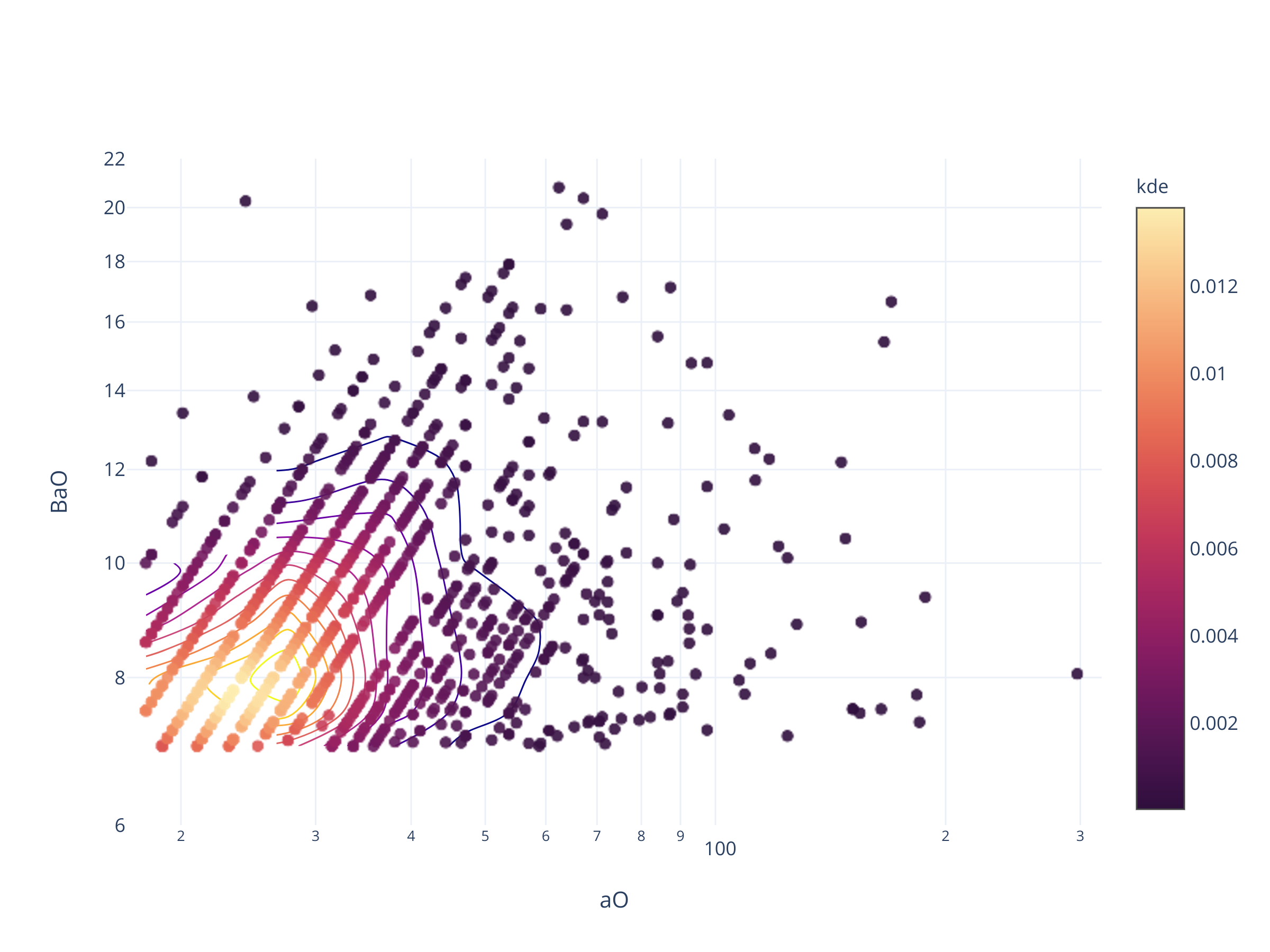
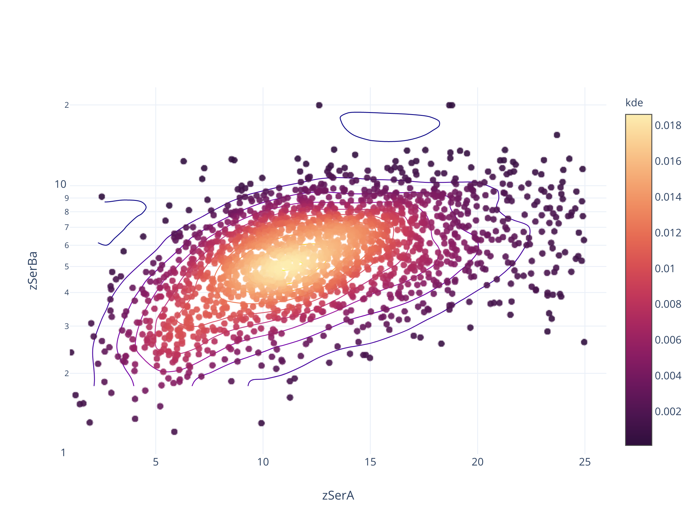
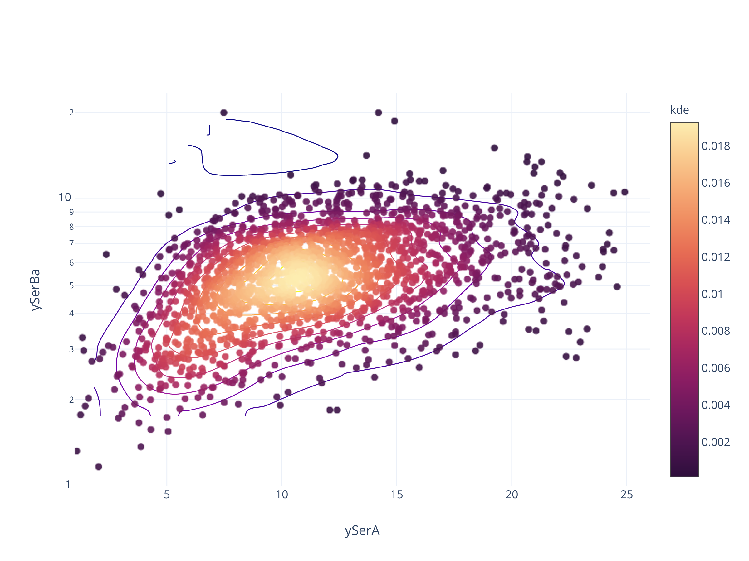
Посмотрим как оно может выглядеть для объектов PanSTARRS

fig = scadensrfgc_ply(
    biggestsermag_aligned, 
    f'{filt}SerA', f'{filt}SerBa',
    (1, 26), (1, 1/0.043)
)
fig.update_layout(autosize=False, width=600, height=500)
fig

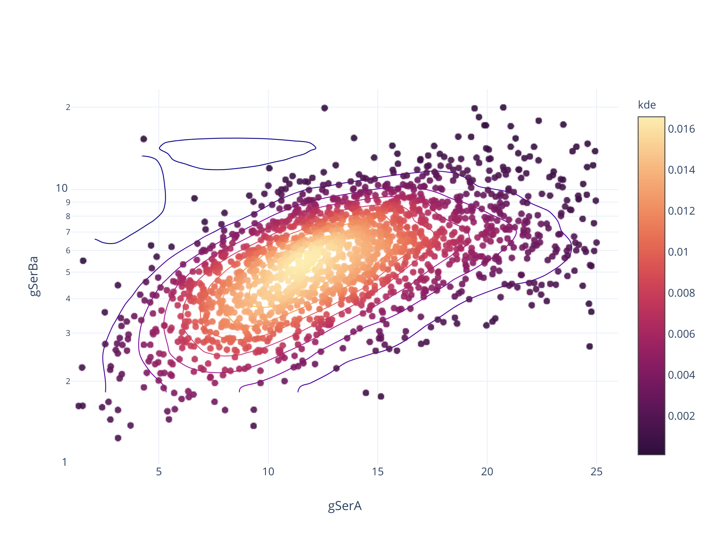
Совсем не так.

В PanSTARRS, судя по всему, есть программный предел в 0.05 и 25.

Отрезать по $a/b > 7$ и $a > 18''$ бессмысленно -- ничего не останется, надо думать

0. Границы по большой полуоси¶

FWHM у PSF в обзоре $1''-2''$ (Глянул у пары галактик, но надо ещё уточнить)

Если у галактики полуось < $7''$, она будет видна с отношением осей $<7$ (а если нет, то это ошибка алгоритма). Получается, что надо отсекать где-то по $5'' - 7''$

t = biggestsermag_aligned
sizemask = {
    5:(t[f'{filt}SerA'] > 5),
    7:(t[f'{filt}SerA'] > 7),
}

summary[filt] = {}

masks_t[filt] = {'all': pd.Series(np.ones(len(t), dtype=bool), index = t.index)}
sqlconds[filt] = {'all':f"{filt}SerRadius > 0.051"}

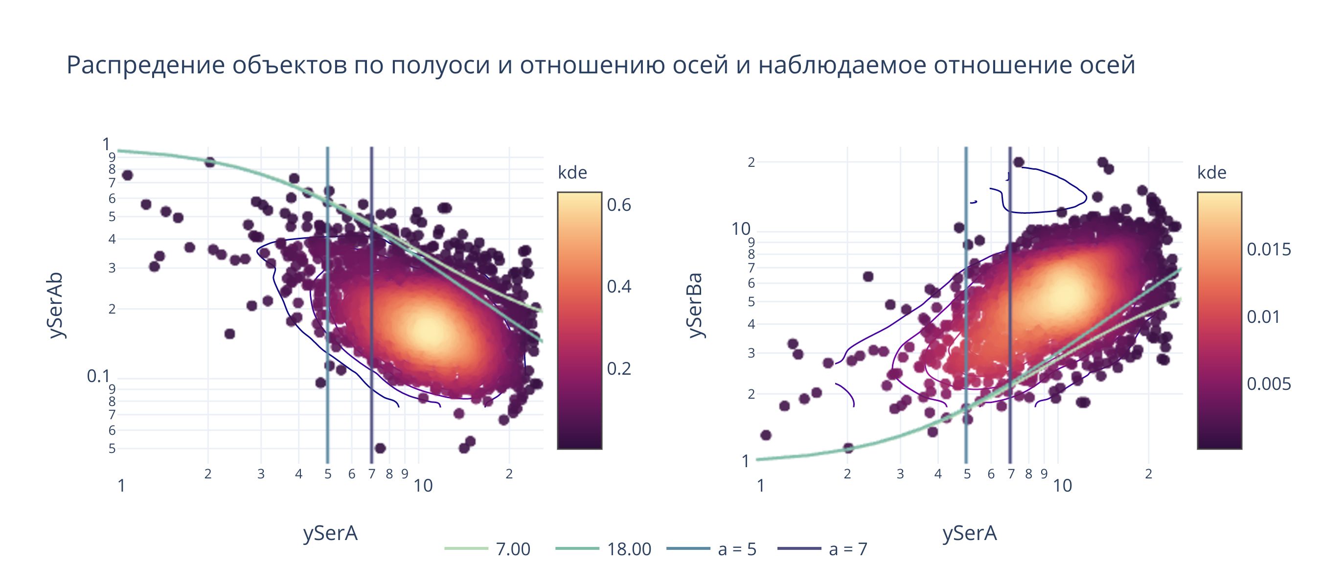
1. По «наблюдаемому» соотношению осей¶

$$ (a/b)_{obs}(a, \sigma) = \frac{\sqrt{a^2 + \sigma^2}}{\sqrt{a^2\,(a/b)^{-2} + \sigma^2}} $$

Можно попробовать подобрать границу «круглости» с помощью этой функции

from code.plotutils import scatter_density_plotly, seaborn_to_plotly

def a_b_obs(a, a_b, sigma=1, inverse=False, ):
    if inverse:
        b = a * (1/a_b)
        ratio = np.sqrt(b**2 + sigma**2) / np.sqrt(a**2 + sigma**2)
    else:
        b = a / a_b
        ratio = np.sqrt(a**2 + sigma**2)/np.sqrt(b**2 + sigma**2) 
    return ratio

def b_a_obs(a, b_a, sigma=1):
    return a_b_obs(a, 1/b_a, sigma, inverse=True)

def _():
    x, y = f'{filt}SerA', f'{filt}SerAb'
    y2 = f'{filt}SerBa'
    xrange, yrange = (1, 26), (0.043, 1) 

    t = biggestsermag_aligned

    mask=(t[x]).between(*xrange) & (t[y].between(*yrange))
    rfgc_names = t.loc[mask, 'RFGC']
    xx = t.loc[mask, x]
    yy = t.loc[mask, y]
    sizes = np.linspace(*xrange, 51)

    a_b_list = np.array([7, 25])
    b_a_list = 1/a_b_list
    N = len(a_b_list)

    plots_kw = dict(mode="kde", modepars={'bins':(30,30)}, contours=True, alpha=0.9,
                    pointlabels=rfgc_names)

    subplotlayout = dict(rows=1, cols=2)
    fig = make_subplots(**subplotlayout)
    fig.layout.update(
        xaxis = {'domain':[0, 0.4]}, 
        xaxis2 = {'domain':[0.6, 1]},
    )
    fig.layout.xaxis.type = 'log'

    fig = scatter_density_plotly(xx, yy, xrange, yrange, x, y, logy=True, logx=True,
                           subplotpos={'row':1, 'col':1}, subplotlyt=subplotlayout,
                           fig=fig, **plots_kw)
    fig = scatter_density_plotly(xx, 1/yy, xrange, (1/yrange[1], 1/yrange[0]), x, y2, logy=True, logx=True,
                           subplotpos={'row':1, 'col':2}, subplotlyt=subplotlayout,
                           fig=fig, **plots_kw)

    fig.update_traces(
        marker = {'colorbar':{'x':0.4}}, 
        selector = {'type':'scattergl'},
        row = 1, col = 1)
    fig.update_traces(
        marker = {'colorbar':{'x':1}}, 
        selector = {'type':'scattergl'},
        row = 1, col = 2)
    fig.update_layout(showlegend=True, legend_orientation="h")


    pallete = sb.cubehelix_palette(4, start=.5, gamma=0.8, rot=-0.7, dark=0.25, light=0.75)
    ply_chx = seaborn_to_plotly(pallete)

    nncurves = len(fig.data)
    for i, a_b in enumerate(a_b_list):
        fig.add_trace(
            go.Scattergl(
                x = sizes,
                y = b_a_obs(sizes, 1/a_b), 
                name="%.2f" % a_b, showlegend=True,
                legendgroup="%.2f" % a_b,
                hoverinfo='name',
                line = {'color':ply_chx[i][1]}
            ), row=1, col=1)
        fig.add_trace(
            go.Scattergl(
                x = sizes,
                y = a_b_obs(sizes, a_b), 
                name = "%.2f" % a_b,
                hoverinfo='name', showlegend=False,
                line = {'color':ply_chx[i][1]}
            ), row=1, col=2)

    for i, x in enumerate([5, 7]):
        fig.add_trace(go.Scattergl(x = [x, x], y = yrange, mode = "lines", line = {'color': ply_chx[i+2][1]}, 
                                 name=f"a = {x}", hoverinfo = "name", legendgroup=f"a = {x}"),
                      row=1, col=1)
        yrange2 = (1/yrange[1], 1/yrange[0])
        fig.add_trace(go.Scattergl(x = [x, x], y = yrange2, mode = "lines", line = {'color': ply_chx[i+2][1]}, 
                                 name=f"a = {x}", hoverinfo="name", showlegend=False),
                      row=1, col=2)


    fig.layout.legend.x = 0.3
    fig.layout.legend.y = -0.2
    fig.layout.legend.tracegroupgap = 30
    fig.layout.title = "Распредение объектов по полуоси и отношению осей и наблюдаемое отношение осей"

    fw = go.FigureWidget(fig)

    @interact(a_b1 = (1, 30, .1), a_b2 = (1, 30, .1), sigma=(1, 10, 0.1))
    def update(a_b1 = 7, a_b2 = 18, sigma=4):
        with fw.batch_update():
            for i, (a_b, inverse) in enumerate([(a_b1, True), (a_b1, False), (a_b2, True), (a_b2, False)],
                    start=nncurves):
                fw.data[i].update(
                     y = a_b_obs(sizes, a_b, sigma, inverse=inverse),
                     name = "%.2f" % a_b)
    return fw
_().show(height = 400, width=900)

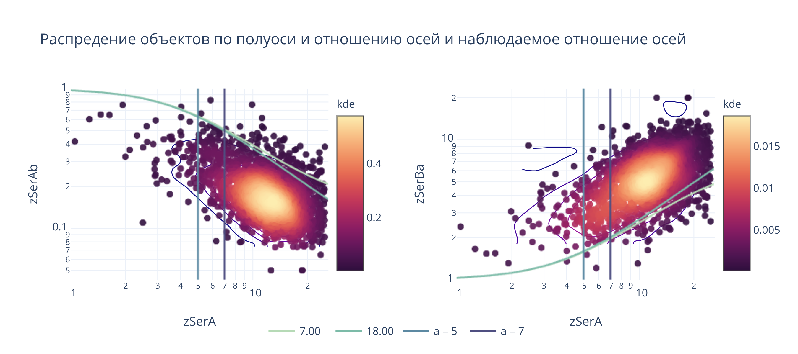
def sel_obs_ratio(t, r_obs, sigma, amin):
    key = f'r_obs={r_obs:d} sigma={sigma:.2f} a>{amin:d}'
    masks_t[filt][key] = (
        (t[f'{filt}SerAb'] < a_b_obs(t[f'{filt}SerA'], r_obs, sigma=sigma, inverse=True)) &
        sizemask[amin]
    )
    sqlconds[filt][key] = f"{filt}SerAb < SQRT(SQUARE({filt}SerRadius/{r_obs:.2f}) + {sigma**2:.2f}) / SQRT(SQUARE({filt}SerRadius) + {sigma**2:.2f}) AND {filt}SerRadius > {amin:.2f}"
sel_obs_ratio(biggestsermag_aligned, 7, 4, 5)    
sel_obs_ratio(biggestsermag_aligned, 7, 4, 7)

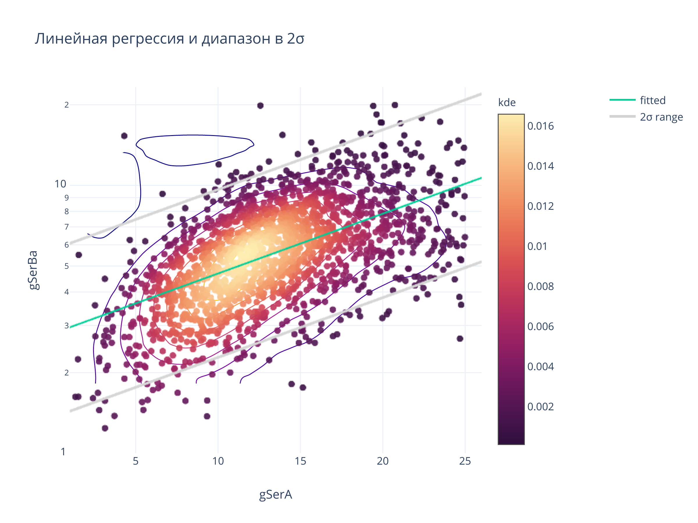
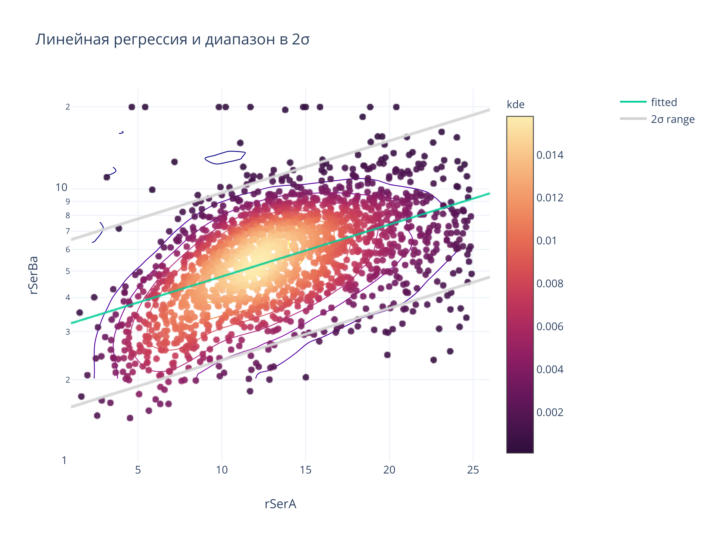
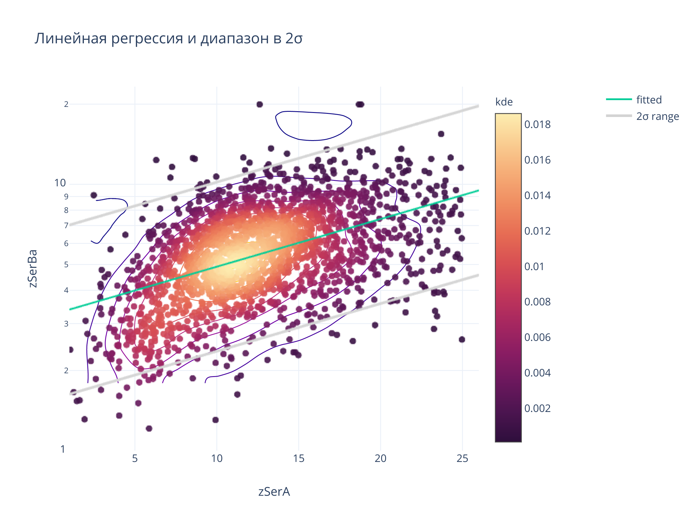
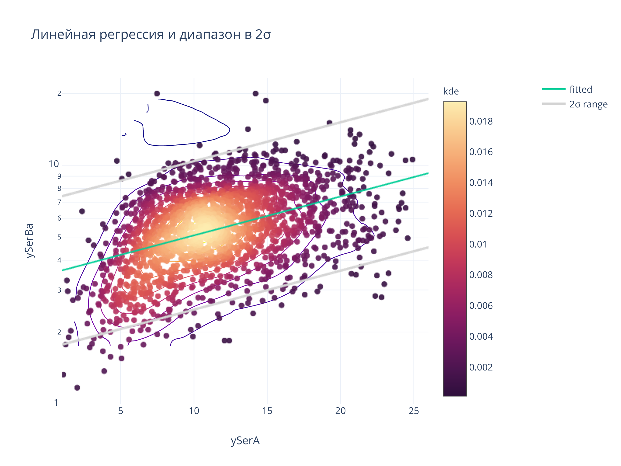
2. По дисперсии линейной регрессии¶

import statsmodels.api as sm
from astropy.modeling import models, fitting

def compute_linregr_pars(t, x, y, xrange, yrange, logx=False, logy=True):
    mask=(t[x]).between(*xrange) & (t[y].between(*yrange))
    xx_reg = (t.loc[mask, x])
    yy_reg = (t.loc[mask, y])
    
    xx_reg = np.log10(xx_reg) if logx else xx_reg
    yy_reg = np.log10(yy_reg) if logy else yy_reg
    
    variables = pd.DataFrame({
        'const':np.ones_like(xx_reg), 
        'x':xx_reg, 
        #'x2':xx**2,
    })

    linmodel = sm.OLS(yy_reg, variables)
    a,b,c,d,e = [0]*5
    mod = Namespace()
    linresults = linmodel.fit()
    mod.eps  = linresults.resid
    mod.b,mod.a = linresults.params
    
    
    hist, xe = np.histogram(mod.eps)
    xe = (xe[1:]+xe[:-1])/2
    
    ini = models.Gaussian1D()
    fitter = fitting.LevMarLSQFitter()
    fit = fitter(ini, xe, hist)
    
    mod.sigma_total = fit.stddev
    return mod

xrange, yrange = (1, 26), (1, 23.26)

m = compute_linregr_pars(
    biggestsermag_aligned,
    f'{filt}SerA', f'{filt}SerBa',
    xrange, yrange
)

x_grid = np.linspace(*xrange, 100)
fitted = 10**(m.a*x_grid + m.b)
upperbnd = 10**(m.a*x_grid + m.b + 2*m.sigma_total)
lowerbnd = 10**(m.a*x_grid + m.b - 2*m.sigma_total)


fig = scadensrfgc_ply(
    biggestsermag_aligned, 
    f'{filt}SerA', f'{filt}SerBa',
    xrange, yrange
)

fig.add_trace(go.Scattergl(x = x_grid, y = fitted, name='fitted'))
fig.add_trace(go.Scattergl(x = np.hstack([x_grid, [x_grid[-1]+1,x_grid[-1]+1], np.flip(x_grid)]), 
                           y = np.hstack([upperbnd, [upperbnd[-1], lowerbnd[-1]], np.flip(lowerbnd)]), line = {'color':'lightgray', 'width':3},
                           name='2σ range'))

fig.layout.legend.x = 1.3
fig.update_layout(
    title = "Линейная регрессия и диапазон в 2σ",
    clickmode = "event+select",
    autosize=False,width=700, height=500)
fig.show()

def sel_lbnd_linreg(t, amin):
    key = f'2 sigma a>{amin:d}'
    masks_t[filt][key] = (
        (np.log10(t[f'{filt}SerBa']) > m.a*t[f'{filt}SerA']+m.b - 2*m.sigma_total) &
        (t[f'{filt}SerA'] > amin)
    )
    sqlconds[filt][key] = f"-LOG10({filt}SerAb) > {m.a:.5f}*gSerRadius + {m.b:.5f} - {2*m.sigma_total:.5f} AND {filt}SerRadius > {amin:.2f}"

#t = biggestsermag_aligned
sel_lbnd_linreg(biggestsermag_aligned, 5)
sel_lbnd_linreg(biggestsermag_aligned, 7)

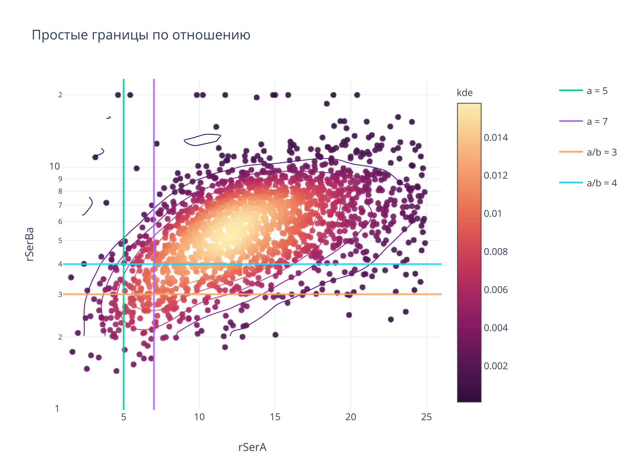
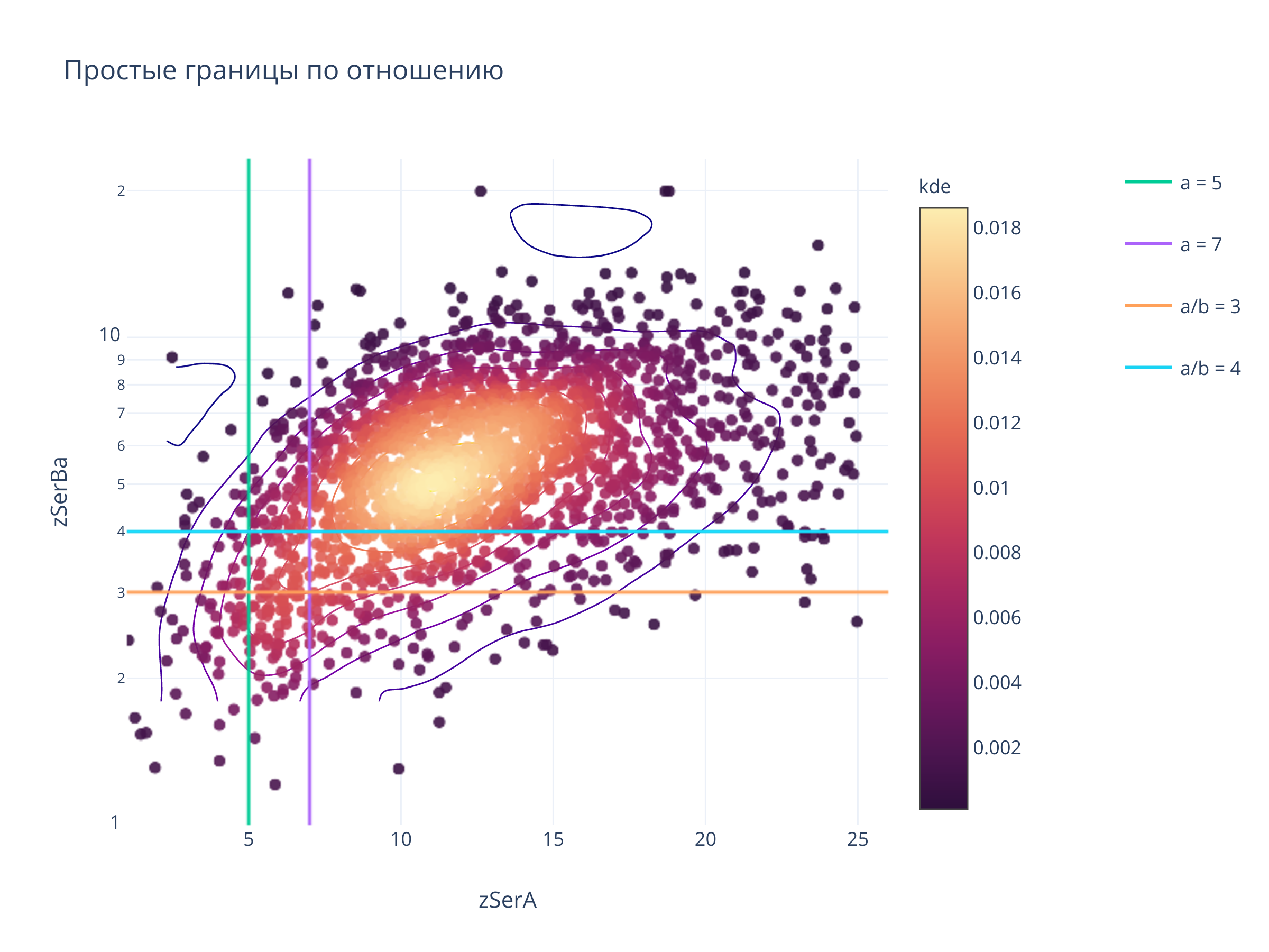
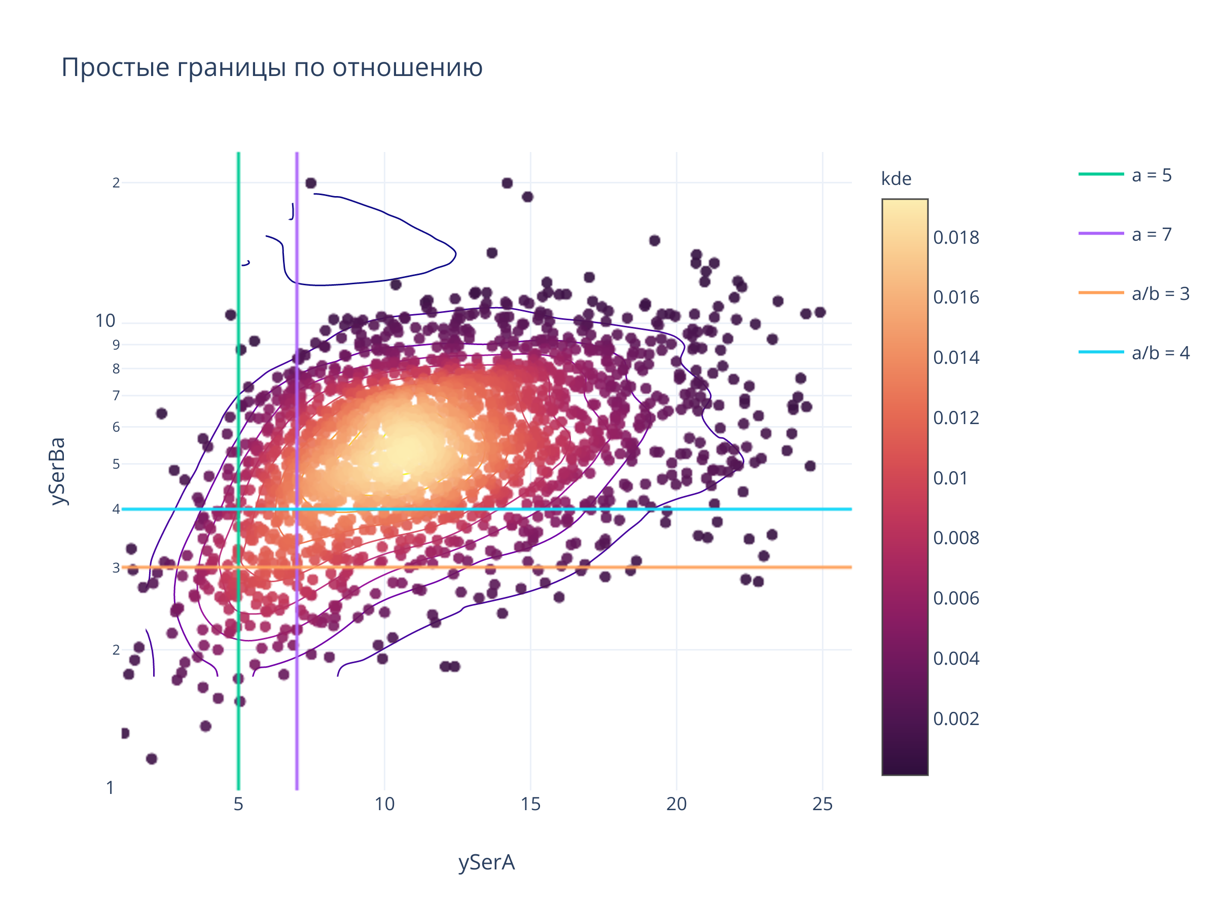
3. Простые границы¶

fig = scadensrfgc_ply(
    biggestsermag_aligned, 
    f'{filt}SerA', f'{filt}SerBa',
    (1, 26), (1, 23.26)
)

x_grid = np.linspace(*xrange, 100)
fig.layout.legend.x = 1.3
fig.layout.legend.tracegroupgap = 20

fig.update_layout(
    title = "Простые границы по отношению",
    clickmode = "event+select",
    autosize=False,width=800, height=600)
for x in [5, 7]:
    fig.add_trace(go.Scattergl(x = [x, x], y = yrange, mode = "lines", name=f"a = {x}", legendgroup=f"a = {x}"))
for y in [3, 4]:
    fig.add_trace(go.Scattergl(x = xrange, y = [y,y],mode = "lines",name=f"a/b = {y}", legendgroup = f"a/b = {y}"))

fig

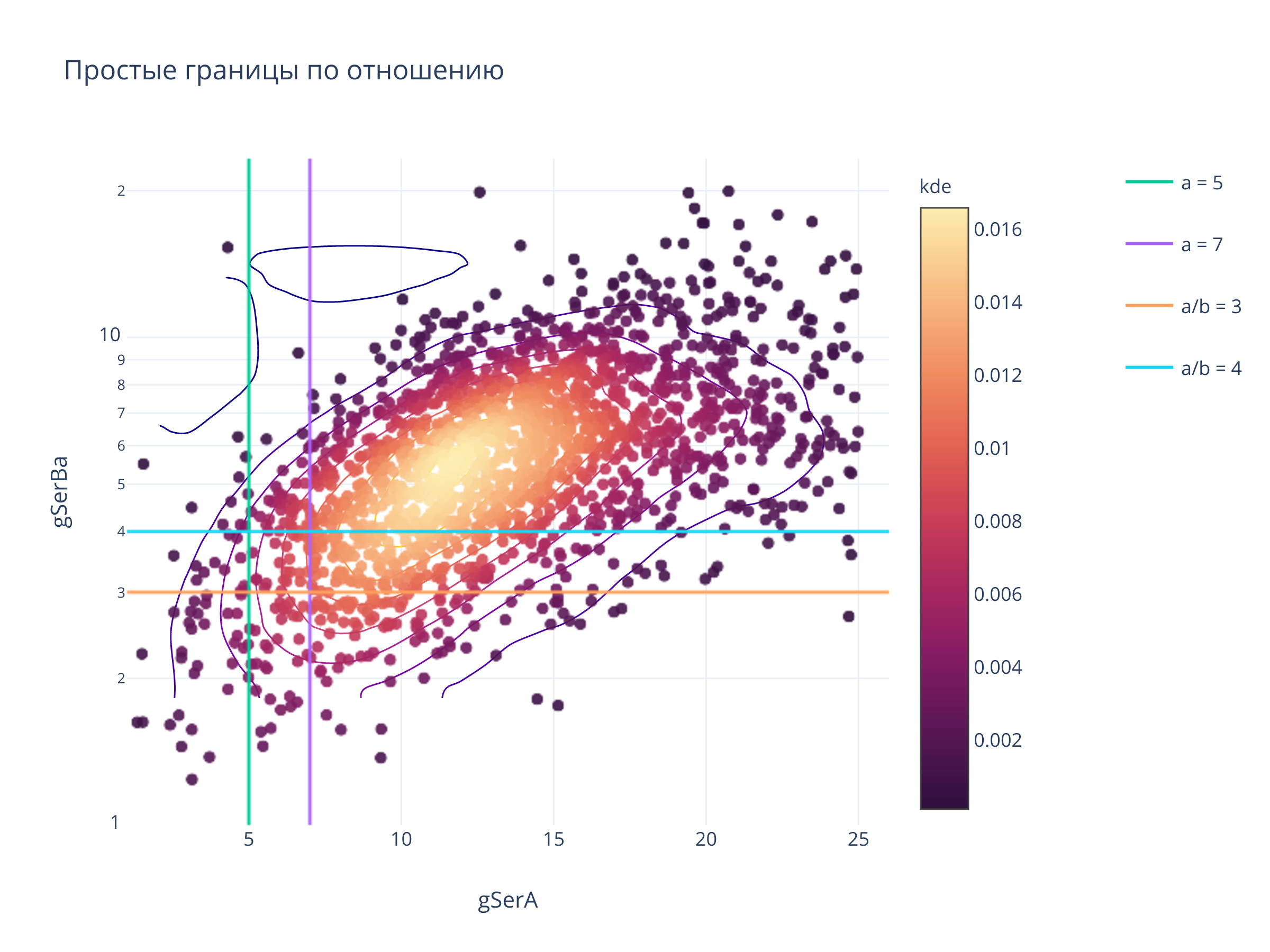
def sel_tresh(t, ratio, amin):
    key = f'a/b>{ratio:d} a>{amin:d}'
    masks_t[filt][key] = (t[f'{filt}SerA'] > amin) & (t[f'{filt}SerBa'] > ratio)
    sqlconds[filt][key] = f"{filt}SerRadius > {amin:.2f} AND {filt}SerAb < {1/ratio:.5f}"
    
sel_tresh(biggestsermag_aligned, 3, 5)
sel_tresh(biggestsermag_aligned, 3, 7)
sel_tresh(biggestsermag_aligned, 4, 5)
sel_tresh(biggestsermag_aligned, 4, 7)

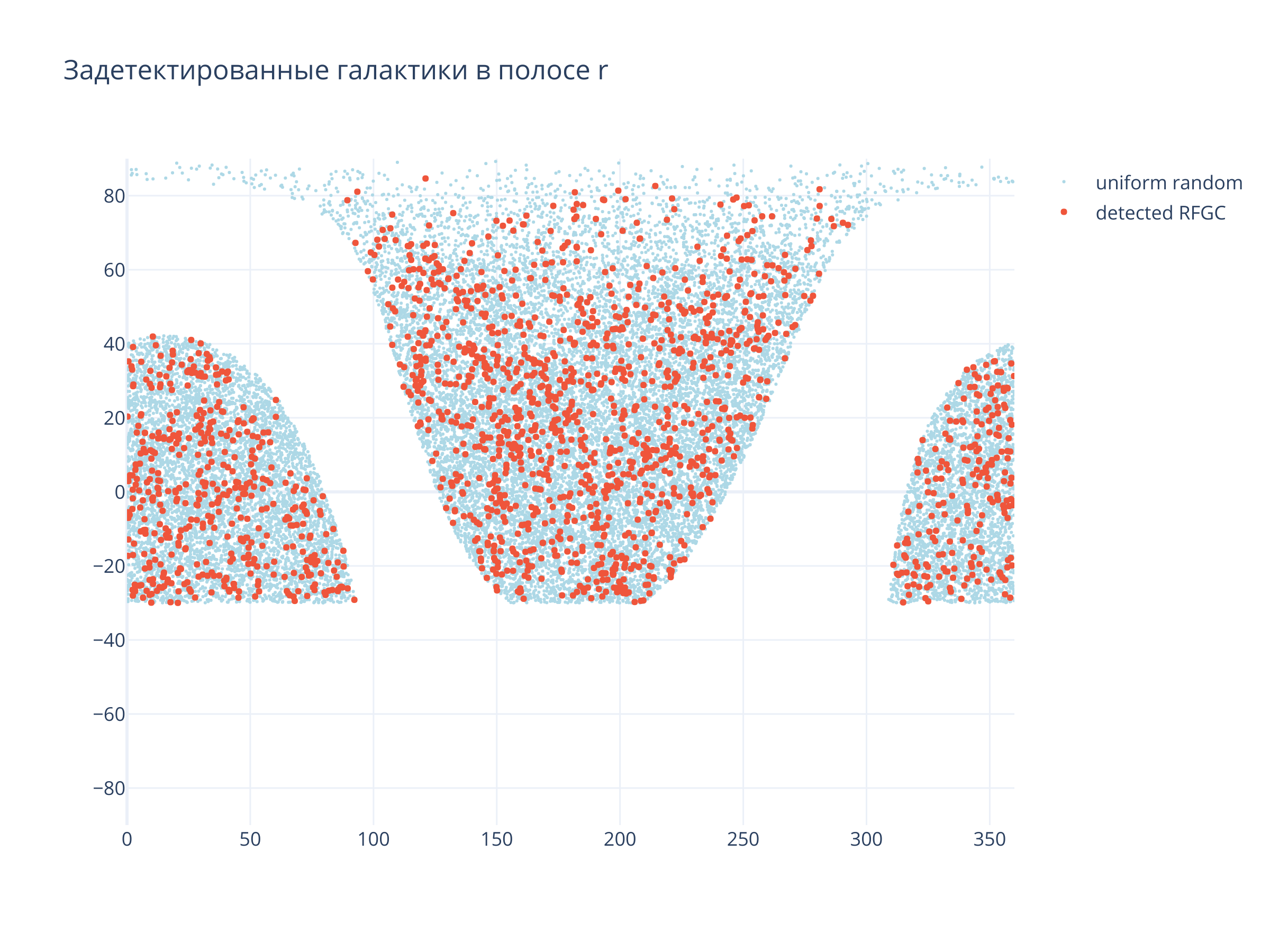
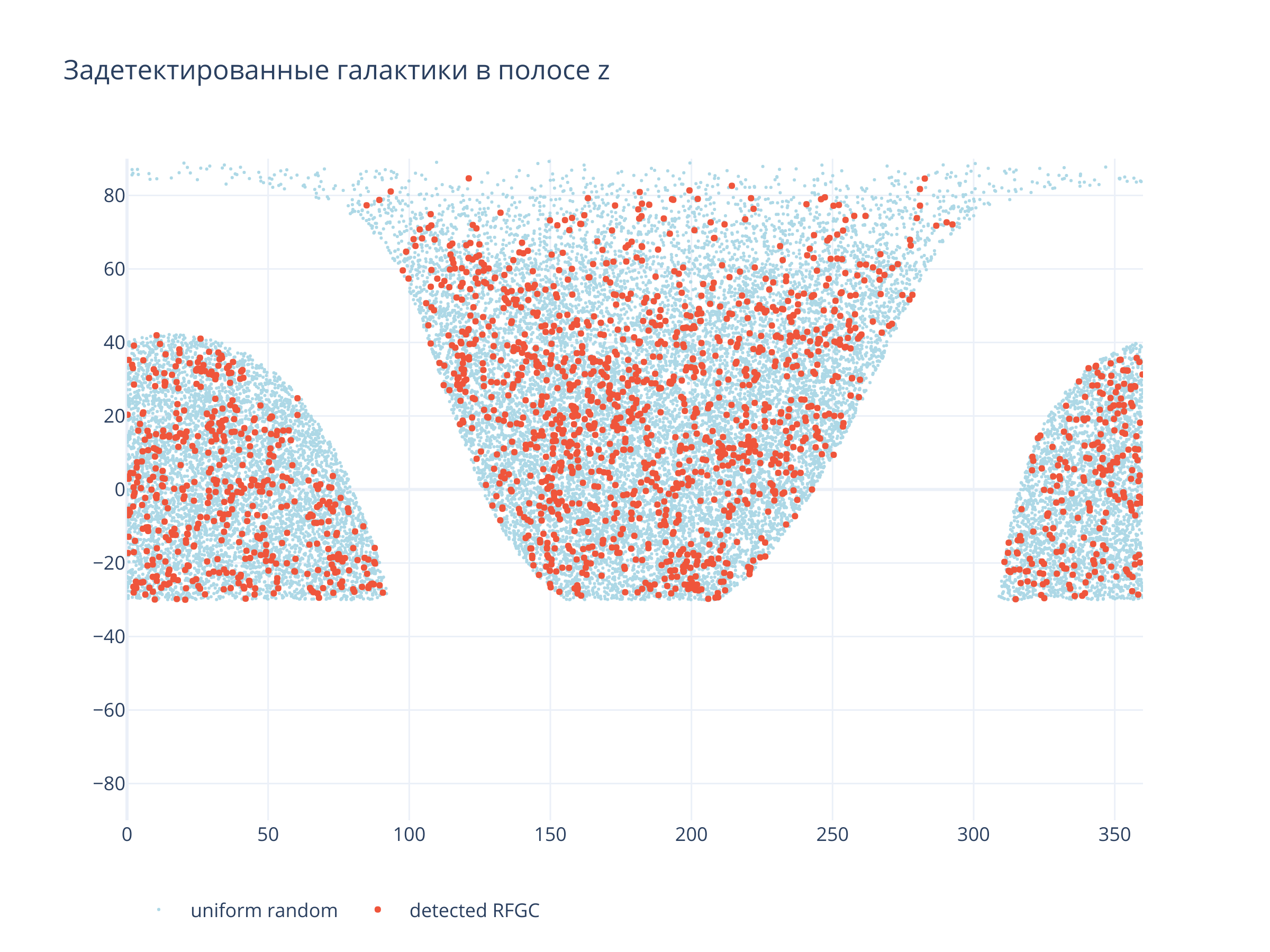
Покрытие неба¶

$$ \begin{aligned} b &> b_0 + r_b \, e^{-\ell^2/(2\sigma_b^2)} \\ b_0 &= 20^\circ \\ r_b &= 15^\circ \\ \sigma_b &= 50^\circ \end{aligned} $$

fig = go.Figure()

fig.add_trace(go.Scatter(
    x = galaxies_sel['ra'],
    y = galaxies_sel['dec'], name = "uniform random",
    hoverinfo = 'none',
    mode = 'markers', marker = {'size': 2, 'color':'lightblue'}
))
fig.add_trace(go.Scatter(
    x = t['RAJ2000'],
    y = t['DEJ2000'], name = "detected RFGC",
    text = list(t['RFGC']),
    hoverinfo = 'text',
    mode = 'markers', marker = {'size': 4}
))


fig.update_layout(
    xaxis = {'range' :[0, 360]},
    yaxis = {'range' :[-90, 90]},
    #width=900, height=700,
    title = f"Задетектированные галактики в полосе {filt}",
    legend_orientation = 'h'
)
    
fig

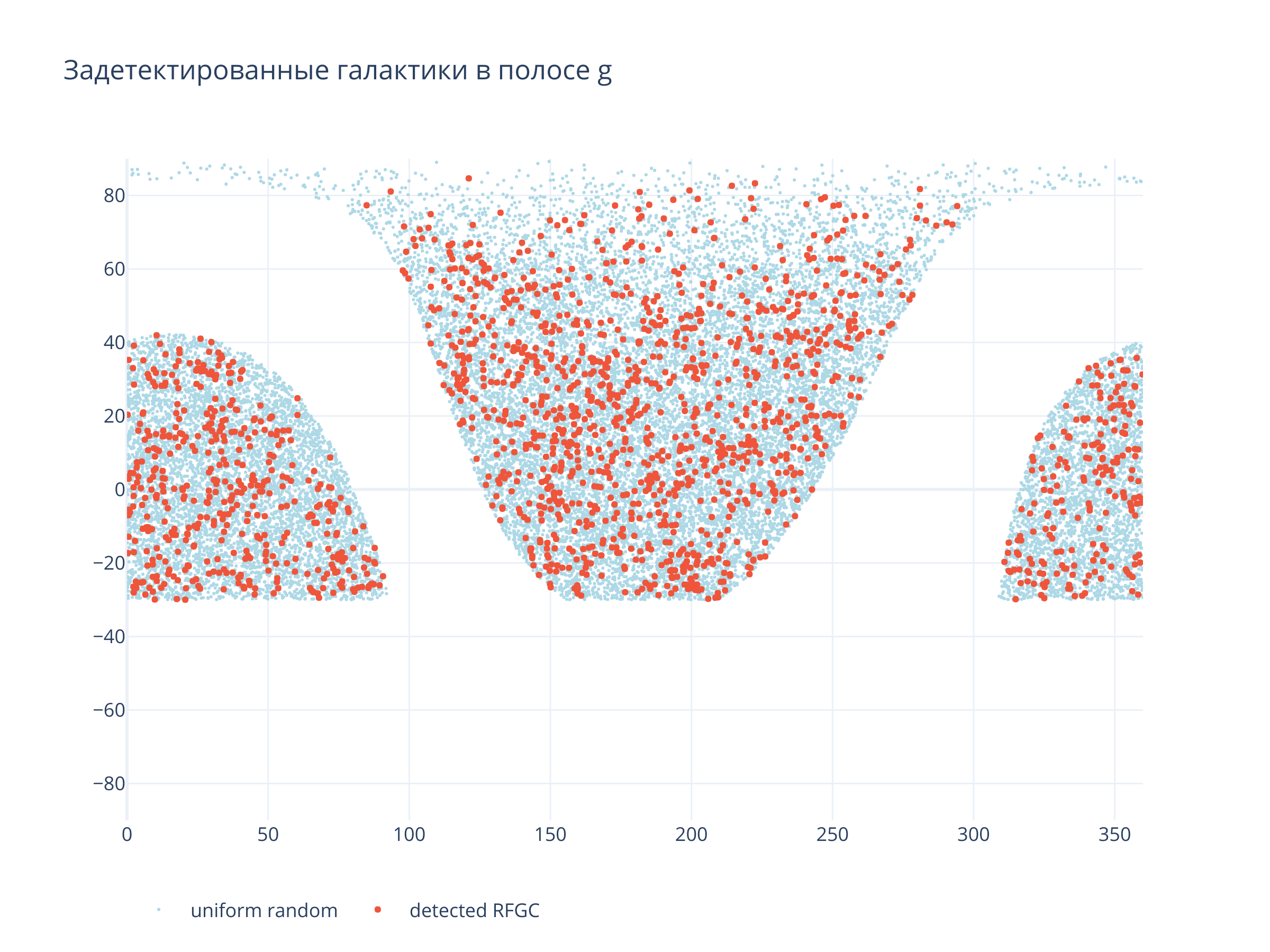
Светло-синие точки --- равномерно распределённые по области детектирования случайные точки

Выводы¶

nrfgc = len(df.drop_duplicates(subset=['RFGC']))

import os
import getpass
if not os.environ.get('CASJOBS_WSID'):
    os.environ['CASJOBS_WSID'] = input('Enter Casjobs WSID (561085547):')
if not os.environ.get('CASJOBS_PW'):
    os.environ['CASJOBS_PW'] = getpass.getpass('Enter Casjobs password:')

import mastcasjobs
jobs = mastcasjobs.MastCasJobs(context="PanSTARRS_DR2", request_type='POST')

from code.hmte import expand_templates
count_template = "".join(open(querypath / 'serscount.tsql').readlines())

@memory.cache
def casquickcaching(jobs, query, task_name):
    res = jobs.quick(query, task_name=task_name)
    return res

@memory.cache
def count_panstarrs(sqlconds, filt):
    r = {}
    for k,v in sqlconds.items():
        whereclause = f"WHERE {v}" if v != "" else ""
        query = expand_templates(count_template, filters=filt, serwhere=whereclause)
        taskname = f"count stuff where {k}"
        try:
            r[k] = (casquickcaching(jobs, query, task_name=taskname))[0][0]
        except Exception as e:
            print(e)
            r[k] = -1
        #r[k] = (jobs.quick(query, task_name=f"count stuff where {k}"))[0][0]
        
        print(whereclause, r[k])
    return r

t = biggestsermag_aligned
def build_summary(t, filt):
    summary = {}
    for k,v in masks_t[filt].items():
        summary[k] = [len(t.loc[v[v].index]), len(t.loc[v[v].index])/nrfgc]
    summary = pd.DataFrame(summary).T
    summary.columns = ['N', 'N/N0']


    summary['N/Nd'] = summary['N'] / (nrfgc * gal_disc_ratio)
    summary['PS'] = np.nan
    
    summary.loc[:, 'PS'] = pd.Series(count_panstarrs(sqlconds[filt], filt))
    
    summary.PS = summary.PS.astype(int)
    summary.N = summary.N.astype(int)
    
    return summary

filt='g'
summary[filt] = build_summary(biggestsermag_aligned, filt)

Таблица¶

Здесь:


N	сколько отобралось объектов, соответствующих галактикам RFGC по критерию
N/N0	доля всего каталога RFGC
N/Nd	c поправкой на неполное покрытие неба
PS	нашлось в PanSTARRS по критерию

summary[filt]

Посмотрим, что не отождествилось вовсе

t1 = df.drop_duplicates(subset=['RFGC'])
t2 = biggestsermag_aligned.drop_duplicates(subset=["RFGC"])
df = pd.concat([t1, t2],sort=True) # concat dataframes
df = df.reset_index(drop=True) # reset the index
df_gpby = df.groupby("RFGC") #group by

idx = [x[0] for x in df_gpby.groups.values() if len(x) == 1] #reindex
unresolved = t1.iloc[idx]

fig = go.Figure()

fig.add_trace(go.Scatter(
    x = galaxies_sel['ra'],
    y = galaxies_sel['dec'], name = "uniform random",
    hoverinfo = 'none',
    mode = 'markers', marker = {'size': 2, 'color':'lightblue'}
))
fig.add_trace(go.Scatter(
    x = unresolved['RAJ2000'],
    y = unresolved['DEJ2000'], name = "unresolved RFGC",
    text = list(unresolved['RFGC']),
    hoverinfo = 'text',
    mode = 'markers', marker = {'size': 4}
))


fig.update_layout(
    xaxis = {'range' :[0, 360]},
    yaxis = {'range' :[-90, 90]},
    height=800,
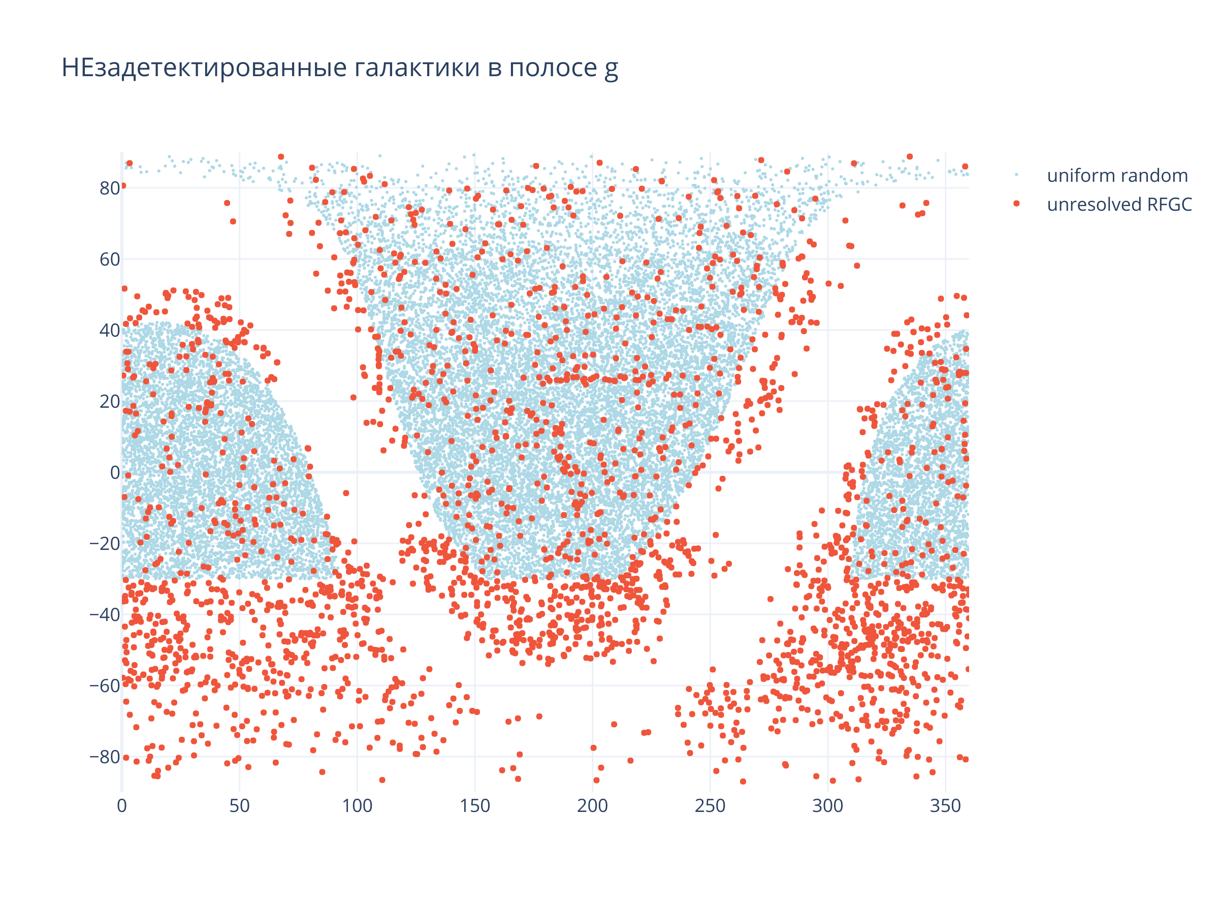
    title = f"НЕзадетектированные галактики в полосе {filt}"
)
    
fig

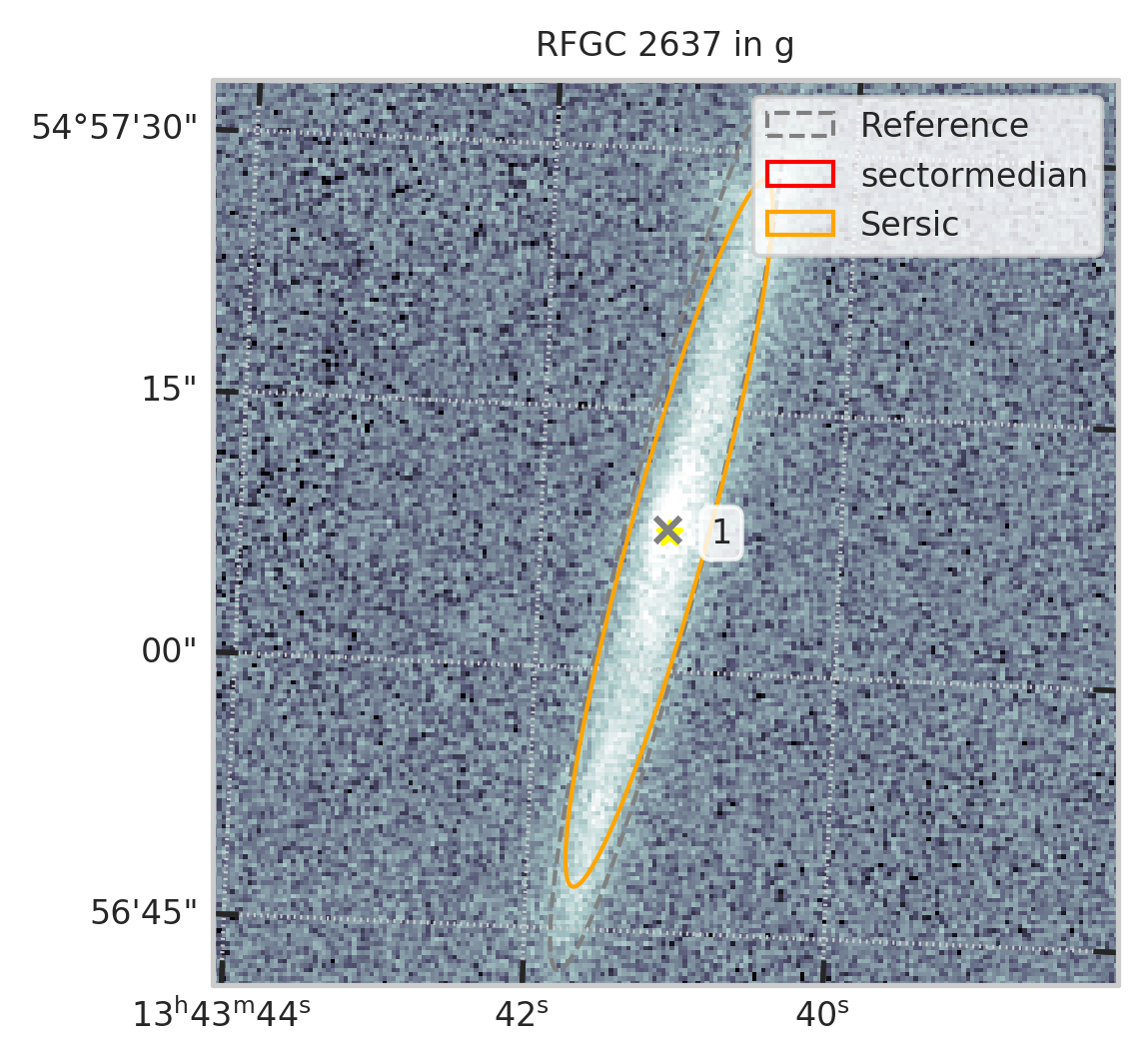
subset = df[df.RFGC == 2637] 
plt.figure(figsize=(4,4))
show_galaxy_rfgc(subset.iloc[0], 'g', df=subset, image=True, fig=fig,
                 sersic=True, cleanp=False, kron=False, median=True, petrosian=False, exp=False, voculer=False,
                 zoom=1, transform=LogStretch(10) + PercentileInterval(99.5))
plt.show()
with pd.option_context("display.max_rows", 1000): display(subset.T)

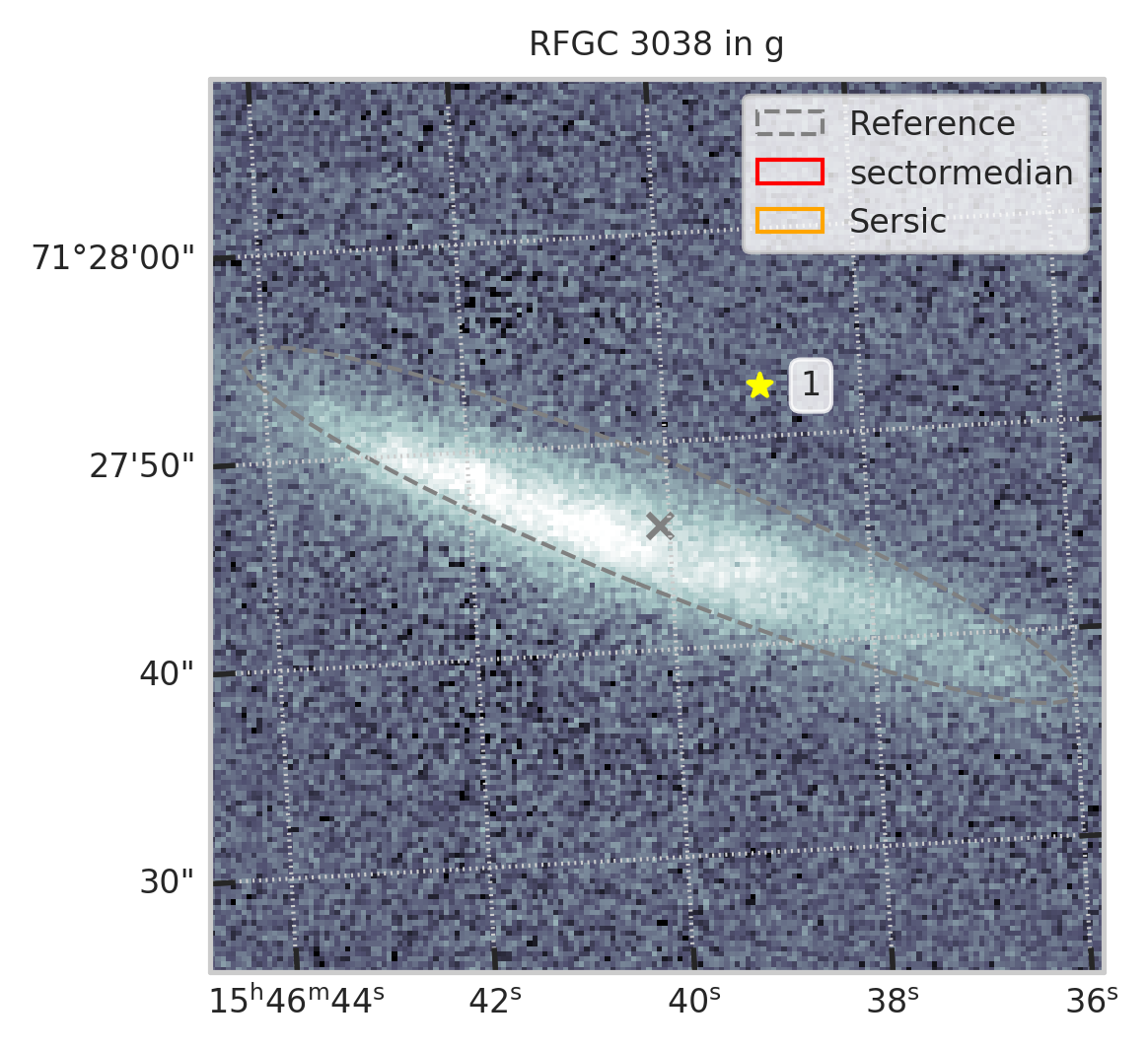
subset = df[df.RFGC == 3038] 
plt.figure(figsize=(4,4))
show_galaxy_rfgc(subset.iloc[0], 'g', df=subset, image=True, fig=fig,
                 sersic=True, cleanp=False, kron=False, median=True, petrosian=False, exp=False, voculer=False,
                 zoom=1, transform=LogStretch(10) + PercentileInterval(99.5))
plt.show()
with pd.option_context("display.max_rows", 1000): display(subset.T)

subset = df[df.RFGC == 509] 
plt.figure(figsize=(4,4))
show_galaxy_rfgc(subset.iloc[0], 'g', df=subset, image=True, fig=fig,
                 sersic=True, cleanp=False, kron=False, median=True, petrosian=False, exp=False, voculer=False,
                 zoom=1, transform=LogStretch(10) + PercentileInterval(99.5))
plt.show()
with pd.option_context("display.max_rows", 1000): display(subset.T)

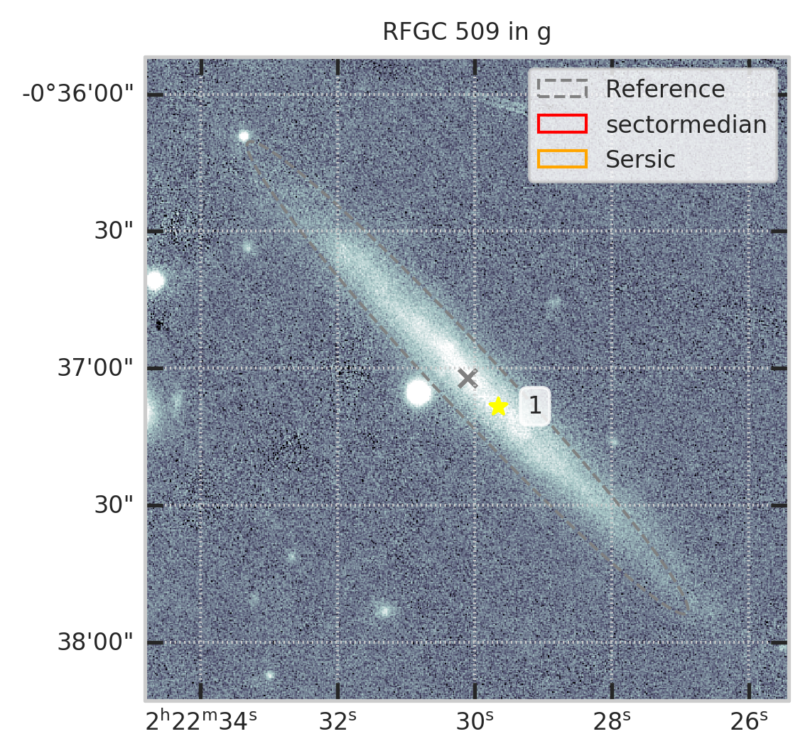
не нашёл он галактику...................

Подбор критериев отбора (r)¶

filt = 'r'

wshape = matches_ref.dropna(subset=[f"{filt}GalIndex"])
fitted = wshape.dropna(subset=[f"{filt}SerRadius"])
sane = fitted[fitted[f"{filt}SerA"] > 0.051]
aligned = sane[(np.abs(sane[f"{filt}GalPhi"] - sane["PA"]) < 10) & \
               (np.abs(sane[f"{filt}SerPhi"] - sane["PA"]) < 10)]

##aligned.index= range(1, len(aligned)+1)
biggestsermag_aligned = aligned.sort_values(["RFGC",f"{filt}SerMag"],ascending=[True, True]).groupby('RFGC').head(1)

t = biggestsermag_aligned
t['BaO'] = 1/t['AbO']
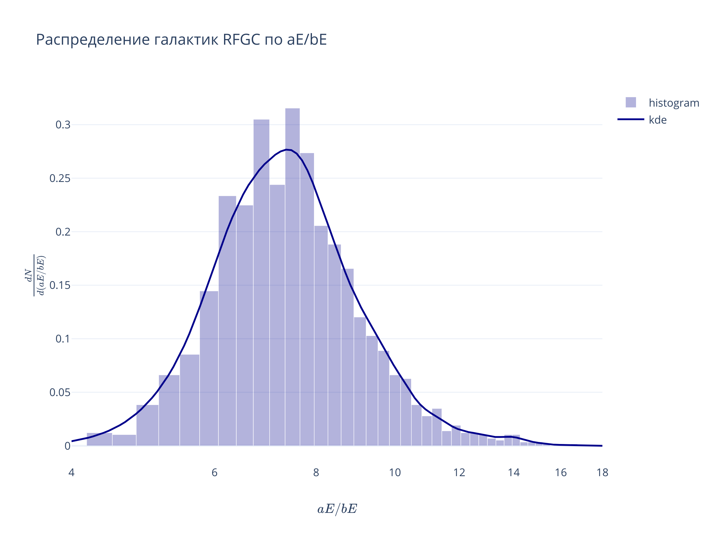
t['AbE'] = t['bE']/t['aE']
t['BaE'] = 1/t['AbE']

from scipy.stats import gaussian_kde

yy, xx_e = np.histogram(t['BaE'], bins='auto', density=True)
xx = (xx_e[1:] + xx_e[:-1])/2

x1, x2 = np.log10(4), np.log10(18)
kernel = gaussian_kde(t['BaE'])
x_grid = np.logspace(x1, x2, 100)

go.Figure(
    data = [
        go.Bar(x = xx, y = yy, width=xx[1]-xx[0], opacity=0.3, marker = {'color':'darkblue'}, name="histogram"),
        go.Scatter(x = x_grid, y = kernel(x_grid), line = {'color':'darkblue'}, name = 'kde')
    ],
    layout = go.Layout(xaxis = {'range':(x1, x2), 'type':'log', 'title':r"$aE/bE$"},
                       yaxis = {'title':r"$\frac{dN}{d (aE/bE)}$"},
                       title="Распределение галактик RFGC по aE/bE")
)

def scadensrfgc_ply(t, x, y, xrange, yrange, **kw):
    
    mask=(t[x]).between(*xrange) & (t[y].between(*yrange))
    rfgc_names = t.loc[mask, 'RFGC']

    xx = t.loc[mask, x]
    yy = t.loc[mask, y]
    #print(len(xx))

    mode = kw.pop('mode', 'kde')
    contours = kw.pop('contours', True)
    logx = kw.pop('logx', False)
    logy = kw.pop('logy', True)
    
    plots_kw = dict(mode=mode, modepars={'bins':(30,30)}, alpha=0.9,
                    pointlabels=rfgc_names, contours=contours, **kw)
    fig = scatter_density_plotly(xx, yy, xrange, yrange, x, y, logy=logy, logx=logx,
                           **plots_kw)
    return fig

fig = scadensrfgc_ply(
    biggestsermag_aligned, 
    'aE', 'BaE', 
    (0.2, 10), (3, 22),
    logx=True
)
fig.update_layout(autosize=False, width=600, height=500)
fig

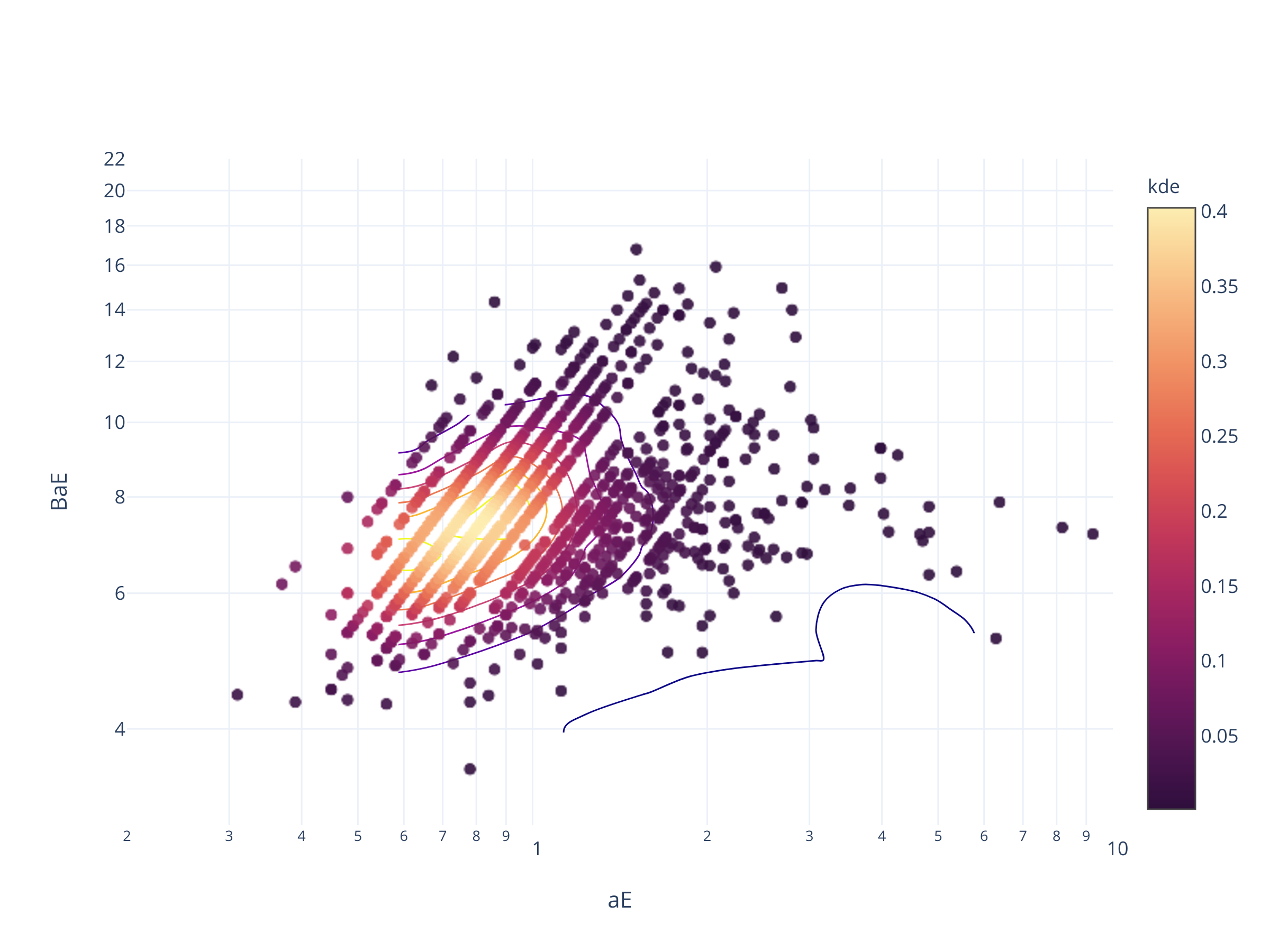
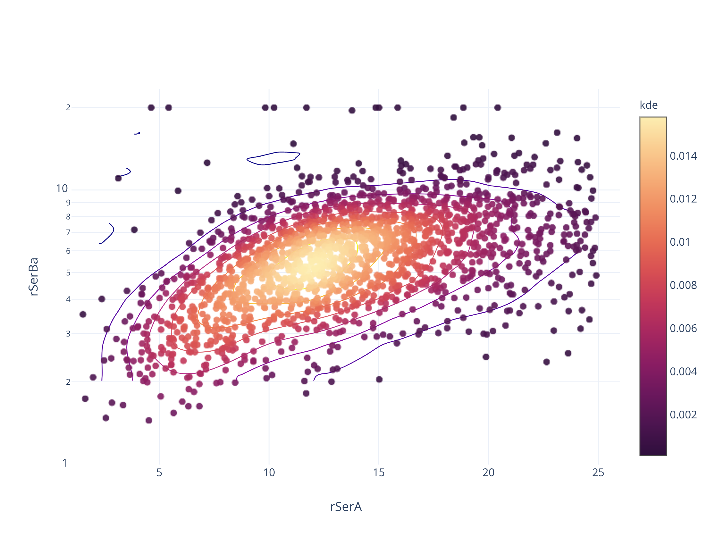
Посмотрим как оно может выглядеть для объектов PanSTARRS

fig = scadensrfgc_ply(
    biggestsermag_aligned, 
    f'{filt}SerA', f'{filt}SerBa',
    (1, 26), (1, 1/0.043)
)
fig.update_layout(autosize=False, width=600, height=500)
fig

0. Границы по большой полуоси¶

FWHM у PSF в обзоре $1''-2''$ (Глянул у пары галактик, но надо ещё уточнить)

Если у галактики полуось < $7''$, она будет видна с отношением осей $<7$ (а если нет, то это ошибка алгоритма). Получается, что надо отсекать где-то по $5'' - 7''$

t = biggestsermag_aligned
sizemask = {
    5:(t[f'{filt}SerA'] > 5),
    7:(t[f'{filt}SerA'] > 7),
}

summary[filt] = {}

masks_t[filt] = {'all': pd.Series(np.ones(len(t), dtype=bool), index = t.index)}
sqlconds[filt] = {'all':f"{filt}SerRadius > 0.051"}

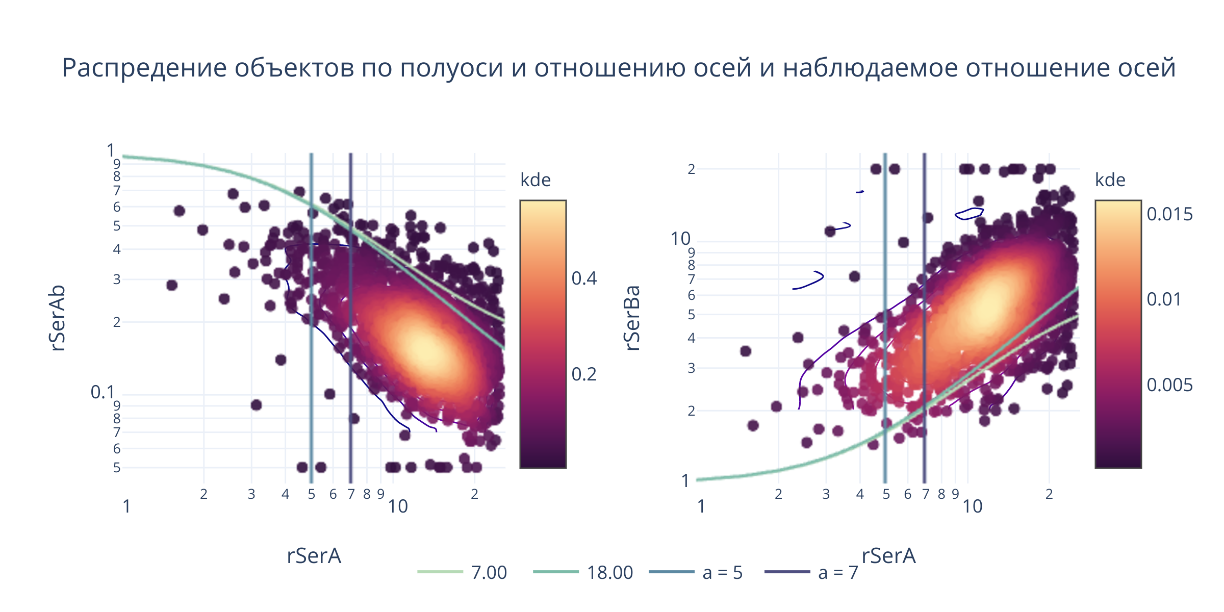
1. По «наблюдаемому» соотношению осей¶

$$ (a/b)_{obs}(a, \sigma) = \frac{\sqrt{a^2 + \sigma^2}}{\sqrt{a^2\,(a/b)^{-2} + \sigma^2}} $$

Можно попробовать подобрать границу «круглости» с помощью этой функции

from code.plotutils import scatter_density_plotly, seaborn_to_plotly

def a_b_obs(a, a_b, sigma=1, inverse=False, ):
    if inverse:
        b = a * (1/a_b)
        ratio = np.sqrt(b**2 + sigma**2) / np.sqrt(a**2 + sigma**2)
    else:
        b = a / a_b
        ratio = np.sqrt(a**2 + sigma**2)/np.sqrt(b**2 + sigma**2) 
    return ratio

def b_a_obs(a, b_a, sigma=1):
    return a_b_obs(a, 1/b_a, sigma, inverse=True)

x, y = f'{filt}SerA', f'{filt}SerAb'
y2 = f'{filt}SerBa'
xrange, yrange = (1, 26), (0.043, 1) 

t = biggestsermag_aligned

mask=(t[x]).between(*xrange) & (t[y].between(*yrange))
rfgc_names = t.loc[mask, 'RFGC']
xx = t.loc[mask, x]
yy = t.loc[mask, y]
sizes = np.linspace(*xrange, 51)

a_b_list = np.array([7, 25])
b_a_list = 1/a_b_list
N = len(a_b_list)

plots_kw = dict(mode="kde", modepars={'bins':(30,30)}, contours=True, alpha=0.9,
                pointlabels=rfgc_names)

subplotlayout = dict(rows=1, cols=2)
fig = make_subplots(**subplotlayout)
fig.layout.update(
    xaxis = {'domain':[0, 0.4]}, 
    xaxis2 = {'domain':[0.6, 1]},
)
fig.layout.xaxis.type = 'log'

fig = scatter_density_plotly(xx, yy, xrange, yrange, x, y, logy=True, logx=True,
                       subplotpos={'row':1, 'col':1}, subplotlyt=subplotlayout,
                       fig=fig, **plots_kw)
fig = scatter_density_plotly(xx, 1/yy, xrange, (1/yrange[1], 1/yrange[0]), x, y2, logy=True, logx=True,
                       subplotpos={'row':1, 'col':2}, subplotlyt=subplotlayout,
                       fig=fig, **plots_kw)

fig.update_traces(
    marker = {'colorbar':{'x':0.4}}, 
    selector = {'type':'scattergl'},
    row = 1, col = 1)
fig.update_traces(
    marker = {'colorbar':{'x':1}}, 
    selector = {'type':'scattergl'},
    row = 1, col = 2)
fig.update_layout(showlegend=True, legend_orientation="h")


pallete = sb.cubehelix_palette(4, start=.5, gamma=0.8, rot=-0.7, dark=0.25, light=0.75)
ply_chx = seaborn_to_plotly(pallete)

nncurves = len(fig.data)
for i, a_b in enumerate(a_b_list):
    fig.add_trace(
        go.Scattergl(
            x = sizes,
            y = b_a_obs(sizes, 1/a_b), 
            name="%.2f" % a_b, showlegend=True,
            legendgroup="%.2f" % a_b,
            hoverinfo='name',
            line = {'color':ply_chx[i][1]}
        ), row=1, col=1)
    fig.add_trace(
        go.Scattergl(
            x = sizes,
            y = a_b_obs(sizes, a_b), 
            name = "%.2f" % a_b,
            hoverinfo='name', showlegend=False,
            line = {'color':ply_chx[i][1]}
        ), row=1, col=2)

for i, x in enumerate([5, 7]):
    fig.add_trace(go.Scattergl(x = [x, x], y = yrange, mode = "lines", line = {'color': ply_chx[i+2][1]}, 
                             name=f"a = {x}", hoverinfo = "name", legendgroup=f"a = {x}"),
                  row=1, col=1)
    yrange2 = (1/yrange[1], 1/yrange[0])
    fig.add_trace(go.Scattergl(x = [x, x], y = yrange2, mode = "lines", line = {'color': ply_chx[i+2][1]}, 
                             name=f"a = {x}", hoverinfo="name", showlegend=False),
                  row=1, col=2)


fig.layout.legend.x = 0.3
fig.layout.legend.y = -0.2
fig.layout.legend.tracegroupgap = 30
fig.layout.title = "Распредение объектов по полуоси и отношению осей и наблюдаемое отношение осей"

fw = go.FigureWidget(fig)

@interact(a_b1 = (1, 30, .1), a_b2 = (1, 30, .1), sigma=(1, 10, 0.1))
def update(a_b1 = 7, a_b2 = 18, sigma=3.8):
    with fw.batch_update():
        for i, (a_b, inverse) in enumerate([(a_b1, True), (a_b1, False), (a_b2, True), (a_b2, False)],
                start=nncurves):
            fw.data[i].update(
                 y = a_b_obs(sizes, a_b, sigma, inverse=inverse),
                 name = "%.2f" % a_b)
fw.show(height=400, width=900)

def sel_obs_ratio(t, r_obs, sigma, amin):
    key = f'r_obs={r_obs:d} sigma={sigma:.2f} a>{amin:d}'
    masks_t[filt][key] = (
        (t[f'{filt}SerAb'] < a_b_obs(t[f'{filt}SerA'], r_obs, sigma=sigma, inverse=True)) &
        sizemask[amin]
    )
    sqlconds[filt][key] = f"{filt}SerAb < SQRT(SQUARE({filt}SerRadius/{r_obs:.2f}) + {sigma**2:.2f}) / SQRT(SQUARE({filt}SerRadius) + {sigma**2:.2f}) AND {filt}SerRadius > {amin:.2f}"
sel_obs_ratio(biggestsermag_aligned, 7, 3.8, 5)    
sel_obs_ratio(biggestsermag_aligned, 7, 3.8, 7)

2. По дисперсии линейной регрессии¶

import statsmodels.api as sm
from astropy.modeling import models, fitting

def compute_linregr_pars(t, x, y, xrange, yrange, logx=False, logy=True):
    mask=(t[x]).between(*xrange) & (t[y].between(*yrange))
    xx_reg = (t.loc[mask, x])
    yy_reg = (t.loc[mask, y])
    
    xx_reg = np.log10(xx_reg) if logx else xx_reg
    yy_reg = np.log10(yy_reg) if logy else yy_reg
    
    variables = pd.DataFrame({
        'const':np.ones_like(xx_reg), 
        'x':xx_reg, 
        #'x2':xx**2,
    })

    linmodel = sm.OLS(yy_reg, variables)
    a,b,c,d,e = [0]*5
    mod = Namespace()
    linresults = linmodel.fit()
    mod.eps  = linresults.resid
    mod.b,mod.a = linresults.params
    
    
    hist, xe = np.histogram(mod.eps)
    xe = (xe[1:]+xe[:-1])/2
    
    ini = models.Gaussian1D()
    fitter = fitting.LevMarLSQFitter()
    fit = fitter(ini, xe, hist)
    
    mod.sigma_total = fit.stddev
    return mod

xrange, yrange = (1, 26), (1, 23.26)

m = compute_linregr_pars(
    biggestsermag_aligned,
    f'{filt}SerA', f'{filt}SerBa',
    xrange, yrange
)

x_grid = np.linspace(*xrange, 100)
fitted = 10**(m.a*x_grid + m.b)
upperbnd = 10**(m.a*x_grid + m.b + 2*m.sigma_total)
lowerbnd = 10**(m.a*x_grid + m.b - 2*m.sigma_total)


fig = scadensrfgc_ply(
    biggestsermag_aligned, 
    f'{filt}SerA', f'{filt}SerBa',
    xrange, yrange
)

fig.add_trace(go.Scattergl(x = x_grid, y = fitted, name='fitted'))
fig.add_trace(go.Scattergl(x = np.hstack([x_grid, [x_grid[-1]+1,x_grid[-1]+1], np.flip(x_grid)]), 
                           y = np.hstack([upperbnd, [upperbnd[-1], lowerbnd[-1]], np.flip(lowerbnd)]), line = {'color':'lightgray', 'width':3},
                           name='2σ range'))

fig.layout.legend.x = 1.3
fig.update_layout(
    title = "Линейная регрессия и диапазон в 2σ",
    clickmode = "event+select",
    autosize=False,width=700, height=500)
fig.show()

def sel_lbnd_linreg(t, amin):
    key = f'2 sigma a>{amin:d}'
    masks_t[filt][key] = (
        (np.log10(t[f'{filt}SerBa']) > m.a*t[f'{filt}SerA']+m.b - 2*m.sigma_total) &
        (t[f'{filt}SerA'] > amin)
    )
    sqlconds[filt][key] = f"-LOG10({filt}SerAb) > {m.a:.5f}*gSerRadius + {m.b:.5f} - {2*m.sigma_total:.5f} AND {filt}SerRadius > {amin:.2f}"

#t = biggestsermag_aligned
sel_lbnd_linreg(biggestsermag_aligned, 5)
sel_lbnd_linreg(biggestsermag_aligned, 7)

3. Простые границы¶

fig = scadensrfgc_ply(
    biggestsermag_aligned, 
    f'{filt}SerA', f'{filt}SerBa',
    (1, 26), (1, 23.26)
)

x_grid = np.linspace(*xrange, 100)
fig.layout.legend.x = 1.3
fig.layout.legend.tracegroupgap = 20

fig.update_layout(
    title = "Простые границы по отношению",
    clickmode = "event+select",
    autosize=False,width=800, height=600)
for x in [5, 7]:
    fig.add_trace(go.Scattergl(x = [x, x], y = yrange, mode = "lines", name=f"a = {x}", legendgroup=f"a = {x}"))
for y in [3, 4]:
    fig.add_trace(go.Scattergl(x = xrange, y = [y,y],mode = "lines",name=f"a/b = {y}", legendgroup = f"a/b = {y}"))

fig

def sel_tresh(t, ratio, amin):
    key = f'a/b>{ratio:d} a>{amin:d}'
    masks_t[filt][key] = ((t[f'{filt}SerA'] > amin) & (t[f'{filt}SerBa'] > ratio))
    sqlconds[filt][key] = f"{filt}SerRadius > {amin:.2f} AND {filt}SerAb < {1/ratio:.5f}"
    
sel_tresh(biggestsermag_aligned, 3, 5)
sel_tresh(biggestsermag_aligned, 3, 7)
sel_tresh(biggestsermag_aligned, 4, 5)
sel_tresh(biggestsermag_aligned, 4, 7)

Покрытие неба¶

$$ \begin{aligned} b &> b_0 + r_b \, e^{-\ell^2/(2\sigma_b^2)} \\ b_0 &= 20^\circ \\ r_b &= 15^\circ \\ \sigma_b &= 50^\circ \end{aligned} $$

fig = go.Figure()

fig.add_trace(go.Scatter(
    x = galaxies_sel['ra'],
    y = galaxies_sel['dec'], name = "uniform random",
    hoverinfo = 'none',
    mode = 'markers', marker = {'size': 2, 'color':'lightblue'}
))
fig.add_trace(go.Scatter(
    x = t['RAJ2000'],
    y = t['DEJ2000'], name = "detected RFGC",
    text = list(t['RFGC']),
    hoverinfo = 'text',
    mode = 'markers', marker = {'size': 4}
))


fig.update_layout(
    xaxis = {'range' :[0, 360]},
    yaxis = {'range' :[-90, 90]},
    height=800,
    title = f"Задетектированные галактики в полосе {filt}"
)
    
fig

Светло-синие точки --- равномерно распределённые по области детектирования случайные точки

Выводы¶

summary[filt] = build_summary(biggestsermag_aligned, filt)

Таблица¶

Здесь:


N	сколько отобралось объектов, соответствующих галактикам RFGC по критерию
N/N0	доля всего каталога RFGC
N/Nd	c поправкой на неполное покрытие неба
PS	нашлось в PanSTARRS по критерию

summary[filt]

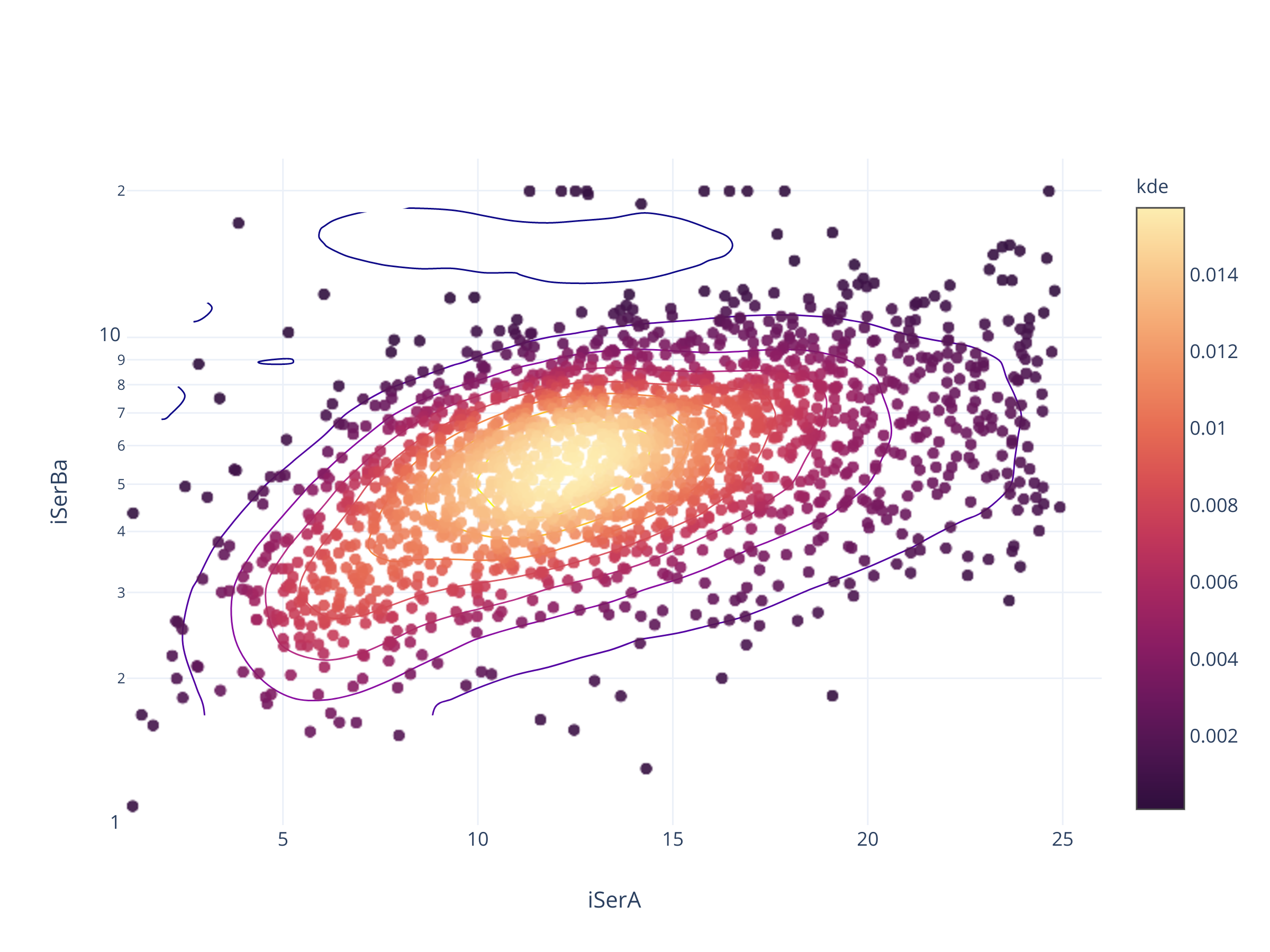
Подбор критериев отбора (i)¶

filt='i'

wshape = matches_ref.dropna(subset=[f"{filt}GalIndex"])
fitted = wshape.dropna(subset=[f"{filt}SerRadius"])
sane = fitted[fitted[f"{filt}SerA"] > 0.051]
aligned = sane[(np.abs(sane[f"{filt}GalPhi"] - sane["PA"]) < 10) & \
               (np.abs(sane[f"{filt}SerPhi"] - sane["PA"]) < 10)]

#aligned.index= range(1, len(aligned)+1)
biggestsermag_aligned = aligned.sort_values(["RFGC",f"{filt}SerMag"],ascending=[True, True]).groupby('RFGC').head(1)

fig = scadensrfgc_ply(
    biggestsermag_aligned, 
    f'{filt}SerA', f'{filt}SerBa',
    (1, 26), (1, 1/0.043)
)
fig.update_layout(autosize=False, width=600, height=500)
fig

0. Границы по большой полуоси¶

FWHM у PSF в обзоре $1''-2''$ (Глянул у пары галактик, но надо ещё уточнить)

Если у галактики полуось < $7''$, она будет видна с отношением осей $<7$ (а если нет, то это ошибка алгоритма). Получается, что надо отсекать где-то по $5'' - 7''$

t = biggestsermag_aligned
sizemask = {
    5:(t[f'{filt}SerA'] > 5),
    7:(t[f'{filt}SerA'] > 7),
}

summary[filt] = {}

masks_t[filt] = {'all': pd.Series(np.ones(len(t), dtype=bool), index=t.index)}
sqlconds[filt] = {'all':f"{filt}SerRadius > 0.051"}

1. По «наблюдаемому» соотношению осей¶

$$ (a/b)_{obs}(a, \sigma) = \frac{\sqrt{a^2 + \sigma^2}}{\sqrt{a^2\,(a/b)^{-2} + \sigma^2}} $$

Можно попробовать подобрать границу «круглости» с помощью этой функции

from code.plotutils import scatter_density_plotly, seaborn_to_plotly

x, y = f'{filt}SerA', f'{filt}SerAb'
y2 = f'{filt}SerBa'
xrange, yrange = (1, 30), (0.043, 1) 

t = biggestsermag_aligned

mask=(t[x]).between(*xrange) & (t[y].between(*yrange))
rfgc_names = t.loc[mask, 'RFGC']
xx = t.loc[mask, x]
yy = t.loc[mask, y]
sizes = np.linspace(*xrange, 51)

a_b_list = np.array([7, 25])
b_a_list = 1/a_b_list
N = len(a_b_list)

plots_kw = dict(mode="kde", modepars={'bins':(30,30)}, contours=True, alpha=0.9,
                pointlabels=rfgc_names)

subplotlayout = dict(rows=1, cols=2)
fig = make_subplots(**subplotlayout)
fig.layout.update(
    xaxis = {'domain':[0, 0.4]}, 
    xaxis2 = {'domain':[0.6, 1]},
)
fig.layout.xaxis.type = 'log'

fig = scatter_density_plotly(xx, yy, xrange, yrange, x, y, logy=True, logx=True,
                       subplotpos={'row':1, 'col':1}, subplotlyt=subplotlayout,
                       fig=fig, **plots_kw)
fig = scatter_density_plotly(xx, 1/yy, xrange, (1/yrange[1], 1/yrange[0]), x, y2, logy=True, logx=True,
                       subplotpos={'row':1, 'col':2}, subplotlyt=subplotlayout,
                       fig=fig, **plots_kw)

fig.update_traces(
    marker = {'colorbar':{'x':0.4}}, 
    selector = {'type':'scattergl'},
    row = 1, col = 1)
fig.update_traces(
    marker = {'colorbar':{'x':1}}, 
    selector = {'type':'scattergl'},
    row = 1, col = 2)
fig.update_layout(showlegend=True, legend_orientation="h")


pallete = sb.cubehelix_palette(4, start=.5, gamma=0.8, rot=-0.7, dark=0.25, light=0.75)
ply_chx = seaborn_to_plotly(pallete)

nncurves = len(fig.data)
for i, a_b in enumerate(a_b_list):
    fig.add_trace(
        go.Scattergl(
            x = sizes,
            y = b_a_obs(sizes, 1/a_b), 
            name="%.2f" % a_b, showlegend=True,
            legendgroup="%.2f" % a_b,
            hoverinfo='name',
            line = {'color':ply_chx[i][1]}
        ), row=1, col=1)
    fig.add_trace(
        go.Scattergl(
            x = sizes,
            y = a_b_obs(sizes, a_b), 
            name = "%.2f" % a_b,
            hoverinfo='name', showlegend=False,
            line = {'color':ply_chx[i][1]}
        ), row=1, col=2)

for i, x in enumerate([5, 7]):
    fig.add_trace(go.Scattergl(x = [x, x], y = yrange, mode = "lines", line = {'color': ply_chx[i+2][1]}, 
                             name=f"a = {x}", hoverinfo = "name", legendgroup=f"a = {x}"),
                  row=1, col=1)
    yrange2 = (1/yrange[1], 1/yrange[0])
    fig.add_trace(go.Scattergl(x = [x, x], y = yrange2, mode = "lines", line = {'color': ply_chx[i+2][1]}, 
                             name=f"a = {x}", hoverinfo="name", showlegend=False),
                  row=1, col=2)


fig.layout.legend.x = 0.3
fig.layout.legend.y = -0.2
fig.layout.legend.tracegroupgap = 30
fig.layout.title = "Распредение объектов по полуоси и отношению осей и наблюдаемое отношение осей"

fw = go.FigureWidget(fig)

@interact(a_b1 = (1, 30, .1), a_b2 = (1, 30, .1), sigma=(1, 10, 0.1))
def update(a_b1 = 7, a_b2 = 18, sigma=3.5):
    with fw.batch_update():
        for i, (a_b, inverse) in enumerate([(a_b1, True), (a_b1, False), (a_b2, True), (a_b2, False)],
                start=nncurves):
            fw.data[i].update(
                 y = a_b_obs(sizes, a_b, sigma, inverse=inverse),
                 name = "%.2f" % a_b)
fw.show(height=400, width=900)

def sel_obs_ratio(t, r_obs, sigma, amin):
    key = f'r_obs={r_obs:d} sigma={sigma:.2f} a>{amin:d}'
    masks_t[filt][key] = (
        (t[f'{filt}SerAb'] < a_b_obs(t[f'{filt}SerA'], r_obs, sigma=sigma, inverse=True)) &
        sizemask[amin]
    )
    sqlconds[filt][key] = f"{filt}SerAb < SQRT(SQUARE({filt}SerRadius/{r_obs:.2f}) + {sigma**2:.2f}) / SQRT(SQUARE({filt}SerRadius) + {sigma**2:.2f}) AND {filt}SerRadius > {amin:.2f}"
sel_obs_ratio(biggestsermag_aligned, 7, 3.5, 5)    
sel_obs_ratio(biggestsermag_aligned, 7, 3.5, 7)

2. По дисперсии линейной регрессии¶

import statsmodels.api as sm
from astropy.modeling import models, fitting

def compute_linregr_pars(t, x, y, xrange, yrange, logx=False, logy=True):
    mask=(t[x]).between(*xrange) & (t[y].between(*yrange))
    xx_reg = (t.loc[mask, x])
    yy_reg = (t.loc[mask, y])
    
    xx_reg = np.log10(xx_reg) if logx else xx_reg
    yy_reg = np.log10(yy_reg) if logy else yy_reg
    
    variables = pd.DataFrame({
        'const':np.ones_like(xx_reg), 
        'x':xx_reg, 
        #'x2':xx**2,
    })

    linmodel = sm.OLS(yy_reg, variables)
    a,b,c,d,e = [0]*5
    mod = Namespace()
    linresults = linmodel.fit()
    mod.eps  = linresults.resid
    mod.b,mod.a = linresults.params
    
    
    hist, xe = np.histogram(mod.eps)
    xe = (xe[1:]+xe[:-1])/2
    
    ini = models.Gaussian1D()
    fitter = fitting.LevMarLSQFitter()
    fit = fitter(ini, xe, hist)
    
    mod.sigma_total = fit.stddev
    return mod

xrange, yrange = (1, 26), (1, 23.26)

m = compute_linregr_pars(
    biggestsermag_aligned,
    f'{filt}SerA', f'{filt}SerBa',
    xrange, yrange
)

x_grid = np.linspace(*xrange, 100)
fitted = 10**(m.a*x_grid + m.b)
upperbnd = 10**(m.a*x_grid + m.b + 2*m.sigma_total)
lowerbnd = 10**(m.a*x_grid + m.b - 2*m.sigma_total)


fig = scadensrfgc_ply(
    biggestsermag_aligned, 
    f'{filt}SerA', f'{filt}SerBa',
    xrange, yrange
)

fig.add_trace(go.Scattergl(x = x_grid, y = fitted, name='fitted'))
fig.add_trace(go.Scattergl(x = np.hstack([x_grid, [x_grid[-1]+1,x_grid[-1]+1], np.flip(x_grid)]), 
                           y = np.hstack([upperbnd, [upperbnd[-1], lowerbnd[-1]], np.flip(lowerbnd)]), line = {'color':'lightgray', 'width':3},
                           name='2σ range'))

fig.layout.legend.x = 1.3
fig.update_layout(
    title = "Линейная регрессия и диапазон в 2σ",
    clickmode = "event+select",
    autosize=False,width=700, height=500)
fig.show()

def sel_lbnd_linreg(t, amin):
    key = f'2 sigma a>{amin:d}'
    masks_t[filt][key] = (
        (np.log10(t[f'{filt}SerBa']) > m.a*t[f'{filt}SerA']+m.b - 2*m.sigma_total) &
        (t[f'{filt}SerA'] > amin)
    )
    sqlconds[filt][key] = f"-LOG10({filt}SerAb) > {m.a:.5f}*gSerRadius + {m.b:.5f} - {2*m.sigma_total:.5f} AND {filt}SerRadius > {amin:.2f}"

#t = biggestsermag_aligned
sel_lbnd_linreg(biggestsermag_aligned, 5)
sel_lbnd_linreg(biggestsermag_aligned, 7)

3. Простые границы¶

fig = scadensrfgc_ply(
    biggestsermag_aligned, 
    f'{filt}SerA', f'{filt}SerBa',
    (1, 26), (1, 23.26)
)

x_grid = np.linspace(*xrange, 100)
fig.layout.legend.x = 1.3
fig.layout.legend.tracegroupgap = 20

fig.update_layout(
    title = "Простые границы по отношению",
    clickmode = "event+select",
    autosize=False,width=800, height=600)
for x in [5, 7]:
    fig.add_trace(go.Scattergl(x = [x, x], y = yrange, mode = "lines", name=f"a = {x}", legendgroup=f"a = {x}"))
for y in [3, 4]:
    fig.add_trace(go.Scattergl(x = xrange, y = [y,y],mode = "lines",name=f"a/b = {y}", legendgroup = f"a/b = {y}"))

fig

def sel_tresh(t, ratio, amin):
    key = f'a/b>{ratio:d} a>{amin:d}'
    masks_t[filt][key] = (t[f'{filt}SerA'] > amin) & (t[f'{filt}SerBa'] > ratio)
    sqlconds[filt][key] = f"{filt}SerRadius > {amin:.2f} AND {filt}SerAb < {1/ratio:.5f}"
    
sel_tresh(biggestsermag_aligned, 3, 5)
sel_tresh(biggestsermag_aligned, 3, 7)
sel_tresh(biggestsermag_aligned, 4, 5)
sel_tresh(biggestsermag_aligned, 4, 7)

Покрытие неба¶

$$ \begin{aligned} b &> b_0 + r_b \, e^{-\ell^2/(2\sigma_b^2)} \\ b_0 &= 20^\circ \\ r_b &= 15^\circ \\ \sigma_b &= 50^\circ \end{aligned} $$

fig = go.Figure()
t = biggestsermag_aligned
fig.add_trace(go.Scatter(
    x = galaxies_sel['ra'],
    y = galaxies_sel['dec'], name = "uniform random",
    hoverinfo = 'none',
    mode = 'markers', marker = {'size': 2, 'color':'lightblue'}
))
fig.add_trace(go.Scatter(
    x = t['RAJ2000'],
    y = t['DEJ2000'], name = "detected RFGC",
    text = list(t['RFGC']),
    hoverinfo = 'text',
    mode = 'markers', marker = {'size': 4}
))


fig.update_layout(
    xaxis = {'range' :[0, 360]},
    yaxis = {'range' :[-90, 90]},
    height=800,
    title = f"Задетектированные галактики в полосе {filt}",
    legend_orientation = 'h'
)
    
fig

Светло-синие точки --- равномерно распределённые по области детектирования случайные точки

Выводы¶

filt = 'i'
summary[filt] = build_summary(biggestsermag_aligned, filt)

/home/iliya/.local/lib/python3.7/site-packages/ipykernel_launcher.py:5: FutureWarning:


Passing list-likes to .loc or [] with any missing label will raise
KeyError in the future, you can use .reindex() as an alternative.

See the documentation here:
https://pandas.pydata.org/pandas-docs/stable/indexing.html#deprecate-loc-reindex-listlike

Таблица¶

Здесь:


N	сколько отобралось объектов, соответствующих галактикам RFGC по критерию
N/N0	доля всего каталога RFGC
N/Nd	c поправкой на неполное покрытие неба
PS	нашлось в PanSTARRS по критерию

summary[filt]

Подбор критериев отбора (z)¶

filt='z'

wshape = matches_ref.dropna(subset=[f"{filt}GalIndex"])
fitted = wshape.dropna(subset=[f"{filt}SerRadius"])
sane = fitted[fitted[f"{filt}SerA"] > 0.051]
aligned = sane[(np.abs(sane[f"{filt}GalPhi"] - sane["PA"]) < 10) & \
               (np.abs(sane[f"{filt}SerPhi"] - sane["PA"]) < 10)]

#aligned.index= range(1, len(aligned)+1)
biggestsermag_aligned = aligned.sort_values(["RFGC",f"{filt}SerMag"],ascending=[True, True]).groupby('RFGC').head(1)

fig = scadensrfgc_ply(
    biggestsermag_aligned, 
    f'{filt}SerA', f'{filt}SerBa',
    (1, 26), (1, 1/0.043)
)
fig.update_layout(autosize=False, width=600, height=500)
fig

0. Границы по большой полуоси¶

FWHM у PSF в обзоре $1''-2''$ (Глянул у пары галактик, но надо ещё уточнить)

Если у галактики полуось < $7''$, она будет видна с отношением осей $<7$ (а если нет, то это ошибка алгоритма). Получается, что надо отсекать где-то по $5'' - 7''$

t = biggestsermag_aligned
sizemask = {
    5:(t[f'{filt}SerA'] > 5),
    7:(t[f'{filt}SerA'] > 7),
}

summary[filt] = {}

masks_t[filt] = {'all': pd.Series(np.ones(len(t), dtype=bool), index=t.index)}
sqlconds[filt] = {'all':f"{filt}SerRadius > 0.051"}

1. По «наблюдаемому» соотношению осей¶

$$ (a/b)_{obs}(a, \sigma) = \frac{\sqrt{a^2 + \sigma^2}}{\sqrt{a^2\,(a/b)^{-2} + \sigma^2}} $$

Можно попробовать подобрать границу «круглости» с помощью этой функции

from code.plotutils import scatter_density_plotly, seaborn_to_plotly

x, y = f'{filt}SerA', f'{filt}SerAb'
y2 = f'{filt}SerBa'
xrange, yrange = (1, 26), (0.043, 1) 

t = biggestsermag_aligned

mask=(t[x]).between(*xrange) & (t[y].between(*yrange))
rfgc_names = t.loc[mask, 'RFGC']
xx = t.loc[mask, x]
yy = t.loc[mask, y]
sizes = np.linspace(*xrange, 51)

a_b_list = np.array([7, 25])
b_a_list = 1/a_b_list
N = len(a_b_list)

plots_kw = dict(mode="kde", modepars={'bins':(30,30)}, contours=True, alpha=0.9,
                pointlabels=rfgc_names)

subplotlayout = dict(rows=1, cols=2)
fig = make_subplots(**subplotlayout)
fig.layout.update(
    xaxis = {'domain':[0, 0.4]}, 
    xaxis2 = {'domain':[0.6, 1]},
)
fig.layout.xaxis.type = 'log'

fig = scatter_density_plotly(xx, yy, xrange, yrange, x, y, logy=True, logx=True,
                       subplotpos={'row':1, 'col':1}, subplotlyt=subplotlayout,
                       fig=fig, **plots_kw)
fig = scatter_density_plotly(xx, 1/yy, xrange, (1/yrange[1], 1/yrange[0]), x, y2, logy=True, logx=True,
                       subplotpos={'row':1, 'col':2}, subplotlyt=subplotlayout,
                       fig=fig, **plots_kw)

fig.update_traces(
    marker = {'colorbar':{'x':0.4}}, 
    selector = {'type':'scattergl'},
    row = 1, col = 1)
fig.update_traces(
    marker = {'colorbar':{'x':1}}, 
    selector = {'type':'scattergl'},
    row = 1, col = 2)
fig.update_layout(showlegend=True, legend_orientation="h")


pallete = sb.cubehelix_palette(4, start=.5, gamma=0.8, rot=-0.7, dark=0.25, light=0.75)
ply_chx = seaborn_to_plotly(pallete)

nncurves = len(fig.data)
for i, a_b in enumerate(a_b_list):
    fig.add_trace(
        go.Scatter(
            x = sizes,
            y = b_a_obs(sizes, 1/a_b), 
            name="%.2f" % a_b, showlegend=True,
            legendgroup="%.2f" % a_b,
            hoverinfo='name',
            line = {'color':ply_chx[i][1]}
        ), row=1, col=1)
    fig.add_trace(
        go.Scatter(
            x = sizes,
            y = a_b_obs(sizes, a_b), 
            name = "%.2f" % a_b,
            hoverinfo='name', showlegend=False,
            line = {'color':ply_chx[i][1]}
        ), row=1, col=2)

for i, x in enumerate([5, 7]):
    fig.add_trace(go.Scattergl(x = [x, x], y = yrange, mode = "lines", line = {'color': ply_chx[i+2][1]}, 
                             name=f"a = {x}", hoverinfo = "name", legendgroup=f"a = {x}"),
                  row=1, col=1)
    yrange2 = (1/yrange[1], 1/yrange[0])
    fig.add_trace(go.Scattergl(x = [x, x], y = yrange2, mode = "lines", line = {'color': ply_chx[i+2][1]}, 
                             name=f"a = {x}", hoverinfo="name", showlegend=False),
                  row=1, col=2)


fig.layout.legend.x = 0.3
fig.layout.legend.y = -0.2
fig.layout.legend.tracegroupgap = 30
fig.layout.title = "Распредение объектов по полуоси и отношению осей и наблюдаемое отношение осей"

fw = go.FigureWidget(fig)

@interact(a_b1 = (1, 30, .1), a_b2 = (1, 30, .1), sigma=(1, 10, 0.1))
def update(a_b1 = 7, a_b2 = 18, sigma=3.5):
    with fw.batch_update():
        for i, (a_b, inverse) in enumerate([(a_b1, True), (a_b1, False), (a_b2, True), (a_b2, False)],
                start=nncurves):
            fw.data[i].update(
                 y = a_b_obs(sizes, a_b, sigma, inverse=inverse),
                 name = "%.2f" % a_b)
fw.show(height=400, width=900)

def sel_obs_ratio(t, r_obs, sigma, amin):
    key = f'r_obs={r_obs:d} sigma={sigma:.2f} a>{amin:d}'
    masks_t[filt][key] = (
        (t[f'{filt}SerAb'] < a_b_obs(t[f'{filt}SerA'], r_obs, sigma=sigma, inverse=True)) &
        sizemask[amin]
    )
    sqlconds[filt][key] = f"{filt}SerAb < SQRT(SQUARE({filt}SerRadius/{r_obs:.2f}) + {sigma**2:.2f}) / SQRT(SQUARE({filt}SerRadius) + {sigma**2:.2f}) AND {filt}SerRadius > {amin:.2f}"
sel_obs_ratio(biggestsermag_aligned, 7, 3.5, 5)    
sel_obs_ratio(biggestsermag_aligned, 7, 3.5, 7)

2. По дисперсии линейной регрессии¶

import statsmodels.api as sm
from astropy.modeling import models, fitting

def compute_linregr_pars(t, x, y, xrange, yrange, logx=False, logy=True):
    mask=(t[x]).between(*xrange) & (t[y].between(*yrange))
    xx_reg = (t.loc[mask, x])
    yy_reg = (t.loc[mask, y])
    
    xx_reg = np.log10(xx_reg) if logx else xx_reg
    yy_reg = np.log10(yy_reg) if logy else yy_reg
    
    variables = pd.DataFrame({
        'const':np.ones_like(xx_reg), 
        'x':xx_reg, 
        #'x2':xx**2,
    })

    linmodel = sm.OLS(yy_reg, variables)
    a,b,c,d,e = [0]*5
    mod = Namespace()
    linresults = linmodel.fit()
    mod.eps  = linresults.resid
    mod.b,mod.a = linresults.params
    
    
    hist, xe = np.histogram(mod.eps)
    xe = (xe[1:]+xe[:-1])/2
    
    ini = models.Gaussian1D()
    fitter = fitting.LevMarLSQFitter()
    fit = fitter(ini, xe, hist)
    
    mod.sigma_total = fit.stddev
    return mod

xrange, yrange = (1, 26), (1, 23.26)

m = compute_linregr_pars(
    biggestsermag_aligned,
    f'{filt}SerA', f'{filt}SerBa',
    xrange, yrange
)

x_grid = np.linspace(*xrange, 100)
fitted = 10**(m.a*x_grid + m.b)
upperbnd = 10**(m.a*x_grid + m.b + 2*m.sigma_total)
lowerbnd = 10**(m.a*x_grid + m.b - 2*m.sigma_total)


fig = scadensrfgc_ply(
    biggestsermag_aligned, 
    f'{filt}SerA', f'{filt}SerBa',
    xrange, yrange
)

fig.add_trace(go.Scattergl(x = x_grid, y = fitted, name='fitted'))
fig.add_trace(go.Scattergl(x = np.hstack([x_grid, [x_grid[-1]+1,x_grid[-1]+1], np.flip(x_grid)]), 
                           y = np.hstack([upperbnd, [upperbnd[-1], lowerbnd[-1]], np.flip(lowerbnd)]), line = {'color':'lightgray', 'width':3},
                           name='2σ range'))

fig.layout.legend.x = 1.3
fig.update_layout(
    title = "Линейная регрессия и диапазон в 2σ",
    clickmode = "event+select",
    autosize=False,width=700, height=500)
fig.show()

def sel_lbnd_linreg(t, amin):
    key = f'2 sigma a>{amin:d}'
    masks_t[filt][key] = (
        (np.log10(t[f'{filt}SerBa']) > m.a*t[f'{filt}SerA']+m.b - 2*m.sigma_total) &
        (t[f'{filt}SerA'] > amin)
    )
    sqlconds[filt][key] = f"-LOG10({filt}SerAb) > {m.a:.5f}*gSerRadius + {m.b:.5f} - {2*m.sigma_total:.5f} AND {filt}SerRadius > {amin:.2f}"

#t = biggestsermag_aligned
sel_lbnd_linreg(biggestsermag_aligned, 5)
sel_lbnd_linreg(biggestsermag_aligned, 7)

3. Простые границы¶

fig = scadensrfgc_ply(
    biggestsermag_aligned, 
    f'{filt}SerA', f'{filt}SerBa',
    (1, 26), (1, 23.26)
)

x_grid = np.linspace(*xrange, 100)
fig.layout.legend.x = 1.3
fig.layout.legend.tracegroupgap = 20

fig.update_layout(
    title = "Простые границы по отношению",
    clickmode = "event+select",
    autosize=False,width=800, height=600)
for x in [5, 7]:
    fig.add_trace(go.Scattergl(x = [x, x], y = yrange, mode = "lines", name=f"a = {x}", legendgroup=f"a = {x}"))
for y in [3, 4]:
    fig.add_trace(go.Scattergl(x = xrange, y = [y,y],mode = "lines",name=f"a/b = {y}", legendgroup = f"a/b = {y}"))

fig

def sel_tresh(t, ratio, amin):
    key = f'a/b>{ratio:d} a>{amin:d}'
    masks_t[filt][key] = (t[f'{filt}SerA'] > amin) & (t[f'{filt}SerBa'] > ratio)
    sqlconds[filt][key] = f"{filt}SerRadius > {amin:.2f} AND {filt}SerAb < {1/ratio:.5f}"
    
sel_tresh(biggestsermag_aligned, 3, 5)
sel_tresh(biggestsermag_aligned, 3, 7)
sel_tresh(biggestsermag_aligned, 4, 5)
sel_tresh(biggestsermag_aligned, 4, 7)

Покрытие неба¶

$$ \begin{aligned} b &> b_0 + r_b \, e^{-\ell^2/(2\sigma_b^2)} \\ b_0 &= 20^\circ \\ r_b &= 15^\circ \\ \sigma_b &= 50^\circ \end{aligned} $$

fig = go.Figure()
t = biggestsermag_aligned
fig.add_trace(go.Scatter(
    x = galaxies_sel['ra'],
    y = galaxies_sel['dec'], name = "uniform random",
    hoverinfo = 'none',
    mode = 'markers', marker = {'size': 2, 'color':'lightblue'}
))
fig.add_trace(go.Scatter(
    x = t['RAJ2000'],
    y = t['DEJ2000'], name = "detected RFGC",
    text = list(t['RFGC']),
    hoverinfo = 'text',
    mode = 'markers', marker = {'size': 4}
))


fig.update_layout(
    xaxis = {'range' :[0, 360]},
    yaxis = {'range' :[-90, 90]},
    height=800,
    title = f"Задетектированные галактики в полосе {filt}",
    legend_orientation = 'h'
)
    
fig

Светло-синие точки --- равномерно распределённые по области детектирования случайные точки

Выводы¶

filt='z'
summary[filt] = build_summary(biggestsermag_aligned, filt)

Таблица¶

Здесь:


N	сколько отобралось объектов, соответствующих галактикам RFGC по критерию
N/N0	доля всего каталога RFGC
N/Nd	c поправкой на неполное покрытие неба
PS	нашлось в PanSTARRS по критерию

summary[filt]

Подбор критериев отбора (y)¶

filt='y'

wshape = matches_ref.dropna(subset=[f"{filt}GalIndex"])
fitted = wshape.dropna(subset=[f"{filt}SerRadius"])
sane = fitted[fitted[f"{filt}SerA"] > 0.051]
aligned = sane[(np.abs(sane[f"{filt}GalPhi"] - sane["PA"]) < 10) & \
               (np.abs(sane[f"{filt}SerPhi"] - sane["PA"]) < 10)]

#aligned.index= range(1, len(aligned)+1)
biggestsermag_aligned = aligned.sort_values(["RFGC",f"{filt}SerMag"],ascending=[True, True]).groupby('RFGC').head(1)

fig = scadensrfgc_ply(
    biggestsermag_aligned, 
    f'{filt}SerA', f'{filt}SerBa',
    (1, 26), (1, 1/0.043)
)
fig.update_layout(autosize=False, width=600, height=500)
fig

0. Границы по большой полуоси¶

FWHM у PSF в обзоре $1''-2''$ (Глянул у пары галактик, но надо ещё уточнить)

Если у галактики полуось < $7''$, она будет видна с отношением осей $<7$ (а если нет, то это ошибка алгоритма). Получается, что надо отсекать где-то по $5'' - 7''$

t = biggestsermag_aligned
sizemask = {
    5:(t[f'{filt}SerA'] > 5),
    7:(t[f'{filt}SerA'] > 7),
}

summary[filt] = {}
masks_t[filt] = {'all': pd.Series(np.ones(len(t), dtype=bool), index=t.index)}
sqlconds[filt] = {'all':f"{filt}SerRadius > 0.051"}

1. По «наблюдаемому» соотношению осей¶

$$ (a/b)_{obs}(a, \sigma) = \frac{\sqrt{a^2 + \sigma^2}}{\sqrt{a^2\,(a/b)^{-2} + \sigma^2}} $$

Можно попробовать подобрать границу «круглости» с помощью этой функции

from code.plotutils import scatter_density_plotly, seaborn_to_plotly

x, y = f'{filt}SerA', f'{filt}SerAb'
y2 = f'{filt}SerBa'
xrange, yrange = (1, 26), (0.043, 1) 

t = biggestsermag_aligned

mask=(t[x]).between(*xrange) & (t[y].between(*yrange))
rfgc_names = t.loc[mask, 'RFGC']
xx = t.loc[mask, x]
yy = t.loc[mask, y]
sizes = np.linspace(*xrange, 51)

a_b_list = np.array([7, 25])
b_a_list = 1/a_b_list
N = len(a_b_list)

plots_kw = dict(mode="kde", modepars={'bins':(30,30)}, contours=True, alpha=0.9,
                pointlabels=rfgc_names)

subplotlayout = dict(rows=1, cols=2)
fig = make_subplots(**subplotlayout)
fig.layout.update(
    xaxis = {'domain':[0, 0.4]}, 
    xaxis2 = {'domain':[0.6, 1]},
)
fig.layout.xaxis.type = 'log'

fig = scatter_density_plotly(xx, yy, xrange, yrange, x, y, logy=True, logx=True,
                       subplotpos={'row':1, 'col':1}, subplotlyt=subplotlayout,
                       fig=fig, **plots_kw)
fig = scatter_density_plotly(xx, 1/yy, xrange, (1/yrange[1], 1/yrange[0]), x, y2, logy=True, logx=True,
                       subplotpos={'row':1, 'col':2}, subplotlyt=subplotlayout,
                       fig=fig, **plots_kw)

fig.update_traces(
    marker = {'colorbar':{'x':0.4}}, 
    selector = {'type':'scattergl'},
    row = 1, col = 1)
fig.update_traces(
    marker = {'colorbar':{'x':1}}, 
    selector = {'type':'scattergl'},
    row = 1, col = 2)
fig.update_layout(showlegend=True, legend_orientation="h")


pallete = sb.cubehelix_palette(4, start=.5, gamma=0.8, rot=-0.7, dark=0.25, light=0.75)
ply_chx = seaborn_to_plotly(pallete)

nncurves = len(fig.data)
for i, a_b in enumerate(a_b_list):
    fig.add_trace(
        go.Scattergl(
            x = sizes,
            y = b_a_obs(sizes, 1/a_b), 
            name="%.2f" % a_b, showlegend=True,
            legendgroup="%.2f" % a_b,
            hoverinfo='name',
            line = {'color':ply_chx[i][1]}
        ), row=1, col=1)
    fig.add_trace(
        go.Scattergl(
            x = sizes,
            y = a_b_obs(sizes, a_b), 
            name = "%.2f" % a_b,
            hoverinfo='name', showlegend=False,
            line = {'color':ply_chx[i][1]}
        ), row=1, col=2)

for i, x in enumerate([5, 7]):
    fig.add_trace(go.Scattergl(x = [x, x], y = yrange, mode = "lines", line = {'color': ply_chx[i+2][1]}, 
                             name=f"a = {x}", hoverinfo = "name", legendgroup=f"a = {x}"),
                  row=1, col=1)
    yrange2 = (1/yrange[1], 1/yrange[0])
    fig.add_trace(go.Scattergl(x = [x, x], y = yrange2, mode = "lines", line = {'color': ply_chx[i+2][1]}, 
                             name=f"a = {x}", hoverinfo="name", showlegend=False),
                  row=1, col=2)


fig.layout.legend.x = 0.3
fig.layout.legend.y = -0.2
fig.layout.legend.tracegroupgap = 30
fig.layout.title = "Распредение объектов по полуоси и отношению осей и наблюдаемое отношение осей"

fw = go.FigureWidget(fig)

@interact(a_b1 = (1, 30, .1), a_b2 = (1, 30, .1), sigma=(1, 10, 0.1))
def update(a_b1 = 7, a_b2 = 18, sigma=3.5):
    with fw.batch_update():
        for i, (a_b, inverse) in enumerate([(a_b1, True), (a_b1, False), (a_b2, True), (a_b2, False)],
                start=nncurves):
            fw.data[i].update(
                 y = a_b_obs(sizes, a_b, sigma, inverse=inverse),
                 name = "%.2f" % a_b)
fw.show(height=400, width=900)

def sel_obs_ratio(t, r_obs, sigma, amin):
    key = f'r_obs={r_obs:d} sigma={sigma:.2f} a>{amin:d}'
    masks_t[filt][key] = (
        (t[f'{filt}SerAb'] < a_b_obs(t[f'{filt}SerA'], r_obs, sigma=sigma, inverse=True)) &
        sizemask[amin]
    )
    sqlconds[filt][key] = f"{filt}SerAb < SQRT(SQUARE({filt}SerRadius/{r_obs:.2f}) + {sigma**2:.2f}) / SQRT(SQUARE({filt}SerRadius) + {sigma**2:.2f}) AND {filt}SerRadius > {amin:.2f}"
sel_obs_ratio(biggestsermag_aligned, 7, 3.5, 5)    
sel_obs_ratio(biggestsermag_aligned, 7, 3.5, 7)

2. По дисперсии линейной регрессии¶

import statsmodels.api as sm
from astropy.modeling import models, fitting

def compute_linregr_pars(t, x, y, xrange, yrange, logx=False, logy=True):
    mask=(t[x]).between(*xrange) & (t[y].between(*yrange))
    xx_reg = (t.loc[mask, x])
    yy_reg = (t.loc[mask, y])
    
    xx_reg = np.log10(xx_reg) if logx else xx_reg
    yy_reg = np.log10(yy_reg) if logy else yy_reg
    
    variables = pd.DataFrame({
        'const':np.ones_like(xx_reg), 
        'x':xx_reg, 
        #'x2':xx**2,
    })

    linmodel = sm.OLS(yy_reg, variables)
    a,b,c,d,e = [0]*5
    mod = Namespace()
    linresults = linmodel.fit()
    mod.eps  = linresults.resid
    mod.b,mod.a = linresults.params
    
    
    hist, xe = np.histogram(mod.eps)
    xe = (xe[1:]+xe[:-1])/2
    
    ini = models.Gaussian1D()
    fitter = fitting.LevMarLSQFitter()
    fit = fitter(ini, xe, hist)
    
    mod.sigma_total = fit.stddev
    return mod

xrange, yrange = (1, 26), (1, 23.26)

m = compute_linregr_pars(
    biggestsermag_aligned,
    f'{filt}SerA', f'{filt}SerBa',
    xrange, yrange
)

x_grid = np.linspace(*xrange, 100)
fitted = 10**(m.a*x_grid + m.b)
upperbnd = 10**(m.a*x_grid + m.b + 2*m.sigma_total)
lowerbnd = 10**(m.a*x_grid + m.b - 2*m.sigma_total)


fig = scadensrfgc_ply(
    biggestsermag_aligned, 
    f'{filt}SerA', f'{filt}SerBa',
    xrange, yrange
)

fig.add_trace(go.Scattergl(x = x_grid, y = fitted, name='fitted'))
fig.add_trace(go.Scattergl(x = np.hstack([x_grid, [x_grid[-1]+1,x_grid[-1]+1], np.flip(x_grid)]), 
                           y = np.hstack([upperbnd, [upperbnd[-1], lowerbnd[-1]], np.flip(lowerbnd)]), line = {'color':'lightgray', 'width':3},
                           name='2σ range'))

fig.layout.legend.x = 1.3
fig.update_layout(
    title = "Линейная регрессия и диапазон в 2σ",
    clickmode = "event+select",
    autosize=False,width=700, height=500)
fig.show()

def sel_lbnd_linreg(t, amin):
    key = f'2 sigma a>{amin:d}'
    masks_t[filt][key] = (
        (np.log10(t[f'{filt}SerBa']) > m.a*t[f'{filt}SerA']+m.b - 2*m.sigma_total) &
        (t[f'{filt}SerA'] > amin)
    )
    sqlconds[filt][key] = f"-LOG10({filt}SerAb) > {m.a:.5f}*gSerRadius + {m.b:.5f} - {2*m.sigma_total:.5f} AND {filt}SerRadius > {amin:.2f}"

#t = biggestsermag_aligned
sel_lbnd_linreg(biggestsermag_aligned, 5)
sel_lbnd_linreg(biggestsermag_aligned, 7)

3. Простые границы¶

fig = scadensrfgc_ply(
    biggestsermag_aligned, 
    f'{filt}SerA', f'{filt}SerBa',
    (1, 26), (1, 23.26)
)

x_grid = np.linspace(*xrange, 100)
fig.layout.legend.x = 1.3
fig.layout.legend.tracegroupgap = 20

fig.update_layout(
    title = "Простые границы по отношению",
    clickmode = "event+select",
    autosize=False,width=800, height=600)
for x in [5, 7]:
    fig.add_trace(go.Scattergl(x = [x, x], y = yrange, mode = "lines", name=f"a = {x}", legendgroup=f"a = {x}"))
for y in [3, 4]:
    fig.add_trace(go.Scattergl(x = xrange, y = [y,y],mode = "lines",name=f"a/b = {y}", legendgroup = f"a/b = {y}"))

fig

def sel_tresh(t, ratio, amin):
    key = f'a/b>{ratio:d} a>{amin:d}'
    masks_t[filt][key] = (t[f'{filt}SerA'] > amin) & (t[f'{filt}SerBa'] > ratio)
    sqlconds[filt][key] = f"{filt}SerRadius > {amin:.2f} AND {filt}SerAb < {1/ratio:.5f}"
    
sel_tresh(biggestsermag_aligned, 3, 5)
sel_tresh(biggestsermag_aligned, 3, 7)
sel_tresh(biggestsermag_aligned, 4, 5)
sel_tresh(biggestsermag_aligned, 4, 7)

Покрытие неба¶

$$ \begin{aligned} b &> b_0 + r_b \, e^{-\ell^2/(2\sigma_b^2)} \\ b_0 &= 20^\circ \\ r_b &= 15^\circ \\ \sigma_b &= 50^\circ \end{aligned} $$

fig = go.Figure()
t = biggestsermag_aligned
fig.add_trace(go.Scatter(
    x = galaxies_sel['ra'],
    y = galaxies_sel['dec'], name = "uniform random",
    hoverinfo = 'none',
    mode = 'markers', marker = {'size': 2, 'color':'lightblue'}
))
fig.add_trace(go.Scatter(
    x = t['RAJ2000'],
    y = t['DEJ2000'], name = "detected RFGC",
    text = list(t['RFGC']),
    hoverinfo = 'text',
    mode = 'markers', marker = {'size': 4}
))


fig.update_layout(
    xaxis = {'range' :[0, 360]},
    yaxis = {'range' :[-90, 90]},
    height=800,
    title = f"Задетектированные галактики в полосе {filt}",
    legend_orientation = 'h'
)
    
fig

Светло-синие точки --- равномерно распределённые по области детектирования случайные точки

Выводы¶

summary[filt] = build_summary(biggestsermag_aligned, filt)

Таблица¶

Здесь:


N	сколько отобралось объектов, соответствующих галактикам RFGC по критерию
N/N0	доля всего каталога RFGC
N/Nd	c поправкой на неполное покрытие неба
PS	нашлось в PanSTARRS по критерию

summary[filt]

Отбор по выполнению критерия в любой полосе¶

bands = list('grizy')

Выберем здесь такие источники, в которые хотя бы в одной полосе вписан Серсик с радиусом выше программного предела

wshape = matches_ref.dropna(subset=[f"{filt}GalIndex" for filt in bands], how='all')
fitted = wshape.dropna(subset=[f"{filt}SerRadius" for filt in bands], how='all')

sane = fitted[(np.any(fitted.loc[:, [f"{filt}SerA" for filt in bands]] > 0.051, axis=1))]

aligned = sane[np.any(
    [
        (np.abs(sane[galphi] - sane['PA']) < 10) & (np.abs(sane[serphi] - sane['PA']) < 10) 
        for galphi, serphi in zip(
            [f"{filt}GalPhi" for filt in bands], 
            [f"{filt}SerPhi" for filt in bands])
    ], axis=0)]

biggestsermag_aligned = aligned.sort_values(
    [ "RFGC", *[f"{filt}SerMag" for filt in bands]],
    ascending=[True, *[True]*len(bands)]
).groupby('RFGC').head(1)

t = biggestsermag_aligned
ids_per_rfgc = t.groupby('RFGC').count()['objName']
ids_per_rfgc.sort_values(ascending=False)[0:10]

RFGC
4234    1
1493    1
1472    1
1474    1
1475    1
1477    1
1478    1
1479    1
1480    1
1481    1
Name: objName, dtype: int64

fig = go.Figure()
t = biggestsermag_aligned
fig.add_trace(go.Scattergl(
    x = galaxies_sel['ra'],
    y = galaxies_sel['dec'], name = "uniform random",
    hoverinfo = 'none',
    mode = 'markers', marker = {'size': 2, 'color':'lightblue'}
))
fig.add_trace(go.Scattergl(
    x = t['RAJ2000'],
    y = t['DEJ2000'], name = "detected RFGC",
    text = list(t['RFGC']),
    hoverinfo = 'text',
    mode = 'markers', marker = {'size': 4}
))


fig.update_layout(
    xaxis = {'range' :[0, 360]},
    yaxis = {'range' :[-90, 90]},
    height=800,
    title = f"Задетектированные галактики"
)
    
None

from functools import reduce
def allbandsclause(s, bands="grizy", clause="OR"):
    return f" {clause} ".join(["(" + s.format(filt=f) + ")" for f in bands])

def clausejoin(bandkeys, clause="OR"):
    return f" {clause} ".join(["(" + sqlconds[k][v] + ")" for k,v in bandkeys.items()])

t = biggestsermag_aligned
sizemask = {
    5:np.any([t[f'{filt}SerA'] > 5 for filt in bands], axis=0),
    7:np.any([t[f'{filt}SerA'] > 7 for filt in bands], axis=0),
}

filt = 'grizy'
sqlconds[filt] = {'all':clausejoin({k:'all' for k in bands})}
sqlconds[filt]['r_obs a>5'] = clausejoin({
    'g':'r_obs=7 sigma=4.00 a>5', 
    'r':'r_obs=7 sigma=3.80 a>5',
    'i':'r_obs=7 sigma=3.50 a>5',
    'z':'r_obs=7 sigma=3.50 a>5',
    'y':'r_obs=7 sigma=3.50 a>5',
})
sqlconds[filt]['r_obs a>7'] = clausejoin({
    'g':'r_obs=7 sigma=4.00 a>7', 
    'r':'r_obs=7 sigma=3.80 a>7',
    'i':'r_obs=7 sigma=3.50 a>7',
    'z':'r_obs=7 sigma=3.50 a>7',
    'y':'r_obs=7 sigma=3.50 a>7',
})
sqlconds[filt]['2 sigma a>5'] = clausejoin({k:'2 sigma a>5' for k in bands})
sqlconds[filt]['2 sigma a>7'] = clausejoin({k:'2 sigma a>7' for k in bands})

sqlconds[filt]['a/b>3 a>5'] = clausejoin({k:'a/b>3 a>5' for k in bands})
sqlconds[filt]['a/b>3 a>7'] = clausejoin({k:'a/b>3 a>7' for k in bands})
sqlconds[filt]['a/b>4 a>5'] = clausejoin({k:'a/b>4 a>5' for k in bands})
sqlconds[filt]['a/b>4 a>7'] = clausejoin({k:'a/b>4 a>7' for k in bands})

import operator
def maskjoin(bandkeys, action=operator.or_):
    return reduce(action, [masks_t[k][v] for k,v in bandkeys.items()])

filt = 'grizy'
masks_t[filt] = {}
masks_t[filt] = {'all': pd.Series(np.ones(len(t), dtype=bool), index=t.index)}
masks_t[filt]['r_obs a>5'] = maskjoin({
    'g':'r_obs=7 sigma=4.00 a>5', 
    'r':'r_obs=7 sigma=3.80 a>5',
    'i':'r_obs=7 sigma=3.50 a>5',
    'z':'r_obs=7 sigma=3.50 a>5',
    'y':'r_obs=7 sigma=3.50 a>5',
})
masks_t[filt]['r_obs a>7'] = maskjoin({
    'g':'r_obs=7 sigma=4.00 a>7', 
    'r':'r_obs=7 sigma=3.80 a>7',
    'i':'r_obs=7 sigma=3.50 a>7',
    'z':'r_obs=7 sigma=3.50 a>7',
    'y':'r_obs=7 sigma=3.50 a>7',
})
masks_t[filt]['2 sigma a>5'] = maskjoin({k:'2 sigma a>5' for k in bands})
masks_t[filt]['2 sigma a>7'] = maskjoin({k:'2 sigma a>7' for k in bands})

masks_t[filt]['a/b>3 a>5'] = maskjoin({k:'a/b>3 a>5' for k in bands})
masks_t[filt]['a/b>3 a>7'] = maskjoin({k:'a/b>3 a>7' for k in bands})
masks_t[filt]['a/b>4 a>5'] = maskjoin({k:'a/b>4 a>5' for k in bands})
masks_t[filt]['a/b>4 a>7'] = maskjoin({k:'a/b>4 a>7' for k in bands})

summary[filt] = {}

Выводы¶

summary[filt] = build_summary(biggestsermag_aligned, 'grizy')

/home/iliya/.local/lib/python3.7/site-packages/ipykernel_launcher.py:5: FutureWarning:


Passing list-likes to .loc or [] with any missing label will raise
KeyError in the future, you can use .reindex() as an alternative.

See the documentation here:
https://pandas.pydata.org/pandas-docs/stable/indexing.html#deprecate-loc-reindex-listlike

Таблица¶

Здесь:


N	сколько отобралось объектов, соответствующих галактикам RFGC по критерию
N/N0	доля всего каталога RFGC
N/Nd	c поправкой на неполное покрытие неба
PS	нашлось в PanSTARRS по критерию

summary[filt].loc['r_obs a>5', 'PS'] = 13849922
summary[filt].loc['r_obs a>7', 'PS'] = 7492787
summary[filt].loc['2 sigma a>5', 'PS'] = 15569760
summary[filt].loc['2 sigma a>7', 'PS'] = 8922280

summary[filt]

Почему тут для всего вместе получается больше 1 я не знаю. Возможно, так случайно получилось из-за неравномерности распределения галактик.

	gSerRadius	gSerAb	gSerPhi	gGalMajor	gGalMinor	gGalPhi
1	0.05000	1.000000	0.000000	0.051137	0.049683	0.000000
2	4.41248	0.349731	28.084499	4.957860	1.733920	28.084499
3	0.05000	1.000000	0.000000	0.051174	0.048299	0.000000
4	0.05000	1.000000	0.000000	0.051240	0.048194	0.000003
5	0.05000	1.000000	0.000000	0.048255	0.048282	0.000000
6	16.97900	0.365735	37.788200	16.917900	6.187470	37.788200

	gSerRadius	gSerAb	gSerPhi	gSerMag	gGalMajor	gGalMinor	gGalPhi	gGalMag
1	15.4189	0.128471	56.322201	17.917200	15.3634	1.97375	56.322201	17.705799
2	13.2388	0.202263	56.666401	16.134899	13.1911	2.66808	56.666401	16.453800

	N	N/N0	N/Nd	PS
all	1836	0.433428	0.937126	194968392
r_obs=7 sigma=4.00 a>5	1702	0.401794	0.868730	4360479
r_obs=7 sigma=4.00 a>7	1615	0.381256	0.824324	2244744
2 sigma a>5	1728	0.407932	0.882001	4417911
2 sigma a>7	1643	0.387866	0.838616	2389130
a/b>3 a>5	1653	0.390227	0.843720	3604785
a/b>3 a>7	1591	0.375590	0.812074	2093708
a/b>4 a>5	1444	0.340888	0.737043	3086334
a/b>4 a>7	1405	0.331681	0.717136	1774503

	1
AB	0.04
AbO	0.091954
Asym	0
BaO	NaN
Btot	16.8
DEJ2000	54.9523
FGC_E_	1661
MType	d
N	0
PA	76
PGC	NaN
RAJ2000	205.921
RFGC	2637
SB	II
aE	0.87
aO	26.1
bE	0.08
bO	2.4
decMean	54.9522
gGalA	NaN
gGalAb	NaN
gGalB	NaN
gGalBa	NaN
gGalFlags	NaN
gGalIndex	NaN
gGalMag	NaN
gGalMajor	NaN
gGalMinor	NaN
gGalPhi	NaN
gSerA	21.0402
gSerAb	0.105849
gSerB	2.22708
gSerBa	9.44742
gSerDec	54.9522
gSerMag	16.4911
gSerPhi	74.6901
gSerRa	205.921
gSerRadius	21.0402
gkronMag	NaN
gkronRadius	NaN
gpetMag	NaN
gpetRadius	NaN
iGalA	NaN
iGalAb	NaN
iGalB	NaN
iGalBa	NaN
iGalFlags	NaN
iGalIndex	NaN
iGalMag	NaN
iGalMajor	NaN
iGalMinor	NaN
iGalPhi	NaN
iSerA	8.67787
iSerAb	0.13996
iSerB	1.21455
iSerBa	7.1449
iSerDec	54.9523
iSerMag	16.3672
iSerPhi	75.2843
iSerRa	205.921
iSerRadius	8.67787
ikronMag	NaN
ikronRadius	NaN
ipetMag	NaN
ipetRadius	NaN
kronRadiusbestDetection	NaN
kronRadiusprimaryDetection	NaN
objID	1.73942e+17
objName	PSO J205.9214+54.9522
petbestDetection	NaN
petprimaryDetection	NaN
rGalA	NaN
rGalAb	NaN
rGalB	NaN
rGalBa	NaN
rGalFlags	NaN
rGalIndex	NaN
rGalMag	NaN
rGalMajor	NaN
rGalMinor	NaN
rGalPhi	NaN
rSerA	NaN
rSerAb	NaN
rSerB	NaN
rSerBa	NaN
rSerDec	NaN
rSerMag	NaN
rSerPhi	NaN
rSerRa	NaN
rSerRadius	NaN
raMean	205.921
rkronMag	NaN
rkronRadius	NaN
rpetMag	NaN
rpetRadius	NaN
serbestDetection	1
serprimaryDetection	1
yGalA	NaN
yGalAb	NaN
yGalB	NaN
yGalBa	NaN
yGalFlags	NaN
yGalIndex	NaN
yGalMag	NaN
yGalMajor	NaN
yGalMinor	NaN
yGalPhi	NaN
ySerA	17.3129
ySerAb	0.101233
ySerB	1.75264
ySerBa	9.8782
ySerDec	54.9523
ySerMag	14.8688
ySerPhi	74.1267
ySerRa	205.921
ySerRadius	17.3129
ykronMag	NaN
ykronRadius	NaN
ypetMag	NaN
ypetRadius	NaN
zGalA	NaN
zGalAb	NaN
zGalB	NaN
zGalBa	NaN
zGalFlags	NaN
zGalIndex	NaN
zGalMag	NaN
zGalMajor	NaN
zGalMinor	NaN
zGalPhi	NaN
zSerA	19.7281
zSerAb	0.105312
zSerB	2.07761
zSerBa	9.49559
zSerDec	54.9522
zSerMag	15.0056
zSerPhi	74.231
zSerRa	205.921
zSerRadius	19.7281
zkronMag	NaN
zkronRadius	NaN
zpetMag	NaN
zpetRadius	NaN

	1
AB	0.13
AbO	0.138889
Asym	1
BaO	NaN
Btot	16.7
DEJ2000	71.4628
FGC_E_	1956
MType	d
N	1
PA	-22
PGC	NaN
RAJ2000	236.667
RFGC	3038
SB	II
aE	0.8
aO	21.6
bE	0.11
bO	3
decMean	71.4646
gGalA	NaN
gGalAb	NaN
gGalB	NaN
gGalBa	NaN
gGalFlags	NaN
gGalIndex	NaN
gGalMag	NaN
gGalMajor	NaN
gGalMinor	NaN
gGalPhi	NaN
gSerA	NaN
gSerAb	NaN
gSerB	NaN
gSerBa	NaN
gSerDec	NaN
gSerMag	NaN
gSerPhi	NaN
gSerRa	NaN
gSerRadius	NaN
gkronMag	NaN
gkronRadius	NaN
gpetMag	NaN
gpetRadius	NaN
iGalA	NaN
iGalAb	NaN
iGalB	NaN
iGalBa	NaN
iGalFlags	NaN
iGalIndex	NaN
iGalMag	NaN
iGalMajor	NaN
iGalMinor	NaN
iGalPhi	NaN
iSerA	NaN
iSerAb	NaN
iSerB	NaN
iSerBa	NaN
iSerDec	NaN
iSerMag	NaN
iSerPhi	NaN
iSerRa	NaN
iSerRadius	NaN
ikronMag	NaN
ikronRadius	NaN
ipetMag	NaN
ipetRadius	NaN
kronRadiusbestDetection	NaN
kronRadiusprimaryDetection	NaN
objID	1.93752e+17
objName	PSO J236.6626+71.4646
petbestDetection	NaN
petprimaryDetection	NaN
rGalA	NaN
rGalAb	NaN
rGalB	NaN
rGalBa	NaN
rGalFlags	NaN
rGalIndex	NaN
rGalMag	NaN
rGalMajor	NaN
rGalMinor	NaN
rGalPhi	NaN
rSerA	NaN
rSerAb	NaN
rSerB	NaN
rSerBa	NaN
rSerDec	NaN
rSerMag	NaN
rSerPhi	NaN
rSerRa	NaN
rSerRadius	NaN
raMean	236.663
rkronMag	NaN
rkronRadius	NaN
rpetMag	NaN
rpetRadius	NaN
serbestDetection	NaN
serprimaryDetection	NaN
yGalA	NaN
yGalAb	NaN
yGalB	NaN
yGalBa	NaN
yGalFlags	NaN
yGalIndex	NaN
yGalMag	NaN
yGalMajor	NaN
yGalMinor	NaN
yGalPhi	NaN
ySerA	NaN
ySerAb	NaN
ySerB	NaN
ySerBa	NaN
ySerDec	NaN
ySerMag	NaN
ySerPhi	NaN
ySerRa	NaN
ySerRadius	NaN
ykronMag	NaN
ykronRadius	NaN
ypetMag	NaN
ypetRadius	NaN
zGalA	NaN
zGalAb	NaN
zGalB	NaN
zGalBa	NaN
zGalFlags	NaN
zGalIndex	NaN
zGalMag	NaN
zGalMajor	NaN
zGalMinor	NaN
zGalPhi	NaN
zSerA	NaN
zSerAb	NaN
zSerB	NaN
zSerBa	NaN
zSerDec	NaN
zSerMag	NaN
zSerPhi	NaN
zSerRa	NaN
zSerRadius	NaN
zkronMag	NaN
zkronRadius	NaN
zpetMag	NaN
zpetRadius	NaN

	1
AB	0.15
AbO	0.093617
Asym	2
BaO	NaN
Btot	15.2
DEJ2000	-0.617242
FGC_E_	283
MType	dm
N	0
PA	-47
PGC	9028
RAJ2000	35.6254
RFGC	509
SB	II
aE	2.02
aO	70.5
bE	0.22
bO	6.6
decMean	-0.618978
gGalA	NaN
gGalAb	NaN
gGalB	NaN
gGalBa	NaN
gGalFlags	NaN
gGalIndex	NaN
gGalMag	NaN
gGalMajor	NaN
gGalMinor	NaN
gGalPhi	NaN
gSerA	NaN
gSerAb	NaN
gSerB	NaN
gSerBa	NaN
gSerDec	NaN
gSerMag	NaN
gSerPhi	NaN
gSerRa	NaN
gSerRadius	NaN
gkronMag	NaN
gkronRadius	NaN
gpetMag	NaN
gpetRadius	NaN
iGalA	NaN
iGalAb	NaN
iGalB	NaN
iGalBa	NaN
iGalFlags	NaN
iGalIndex	NaN
iGalMag	NaN
iGalMajor	NaN
iGalMinor	NaN
iGalPhi	NaN
iSerA	NaN
iSerAb	NaN
iSerB	NaN
iSerBa	NaN
iSerDec	NaN
iSerMag	NaN
iSerPhi	NaN
iSerRa	NaN
iSerRadius	NaN
ikronMag	NaN
ikronRadius	NaN
ipetMag	NaN
ipetRadius	NaN
kronRadiusbestDetection	NaN
kronRadiusprimaryDetection	NaN
objID	1.0725e+17
objName	PSO J035.6236-00.6190
petbestDetection	NaN
petprimaryDetection	NaN
rGalA	NaN
rGalAb	NaN
rGalB	NaN
rGalBa	NaN
rGalFlags	NaN
rGalIndex	NaN
rGalMag	NaN
rGalMajor	NaN
rGalMinor	NaN
rGalPhi	NaN
rSerA	NaN
rSerAb	NaN
rSerB	NaN
rSerBa	NaN
rSerDec	NaN
rSerMag	NaN
rSerPhi	NaN
rSerRa	NaN
rSerRadius	NaN
raMean	35.6236
rkronMag	NaN
rkronRadius	NaN
rpetMag	NaN
rpetRadius	NaN
serbestDetection	NaN
serprimaryDetection	NaN
yGalA	NaN
yGalAb	NaN
yGalB	NaN
yGalBa	NaN
yGalFlags	NaN
yGalIndex	NaN
yGalMag	NaN
yGalMajor	NaN
yGalMinor	NaN
yGalPhi	NaN
ySerA	NaN
ySerAb	NaN
ySerB	NaN
ySerBa	NaN
ySerDec	NaN
ySerMag	NaN
ySerPhi	NaN
ySerRa	NaN
ySerRadius	NaN
ykronMag	NaN
ykronRadius	NaN
ypetMag	NaN
ypetRadius	NaN
zGalA	NaN
zGalAb	NaN
zGalB	NaN
zGalBa	NaN
zGalFlags	NaN
zGalIndex	NaN
zGalMag	NaN
zGalMajor	NaN
zGalMinor	NaN
zGalPhi	NaN
zSerA	NaN
zSerAb	NaN
zSerB	NaN
zSerBa	NaN
zSerDec	NaN
zSerMag	NaN
zSerPhi	NaN
zSerRa	NaN
zSerRadius	NaN
zkronMag	NaN
zkronRadius	NaN
zpetMag	NaN
zpetRadius	NaN

	N	N/N0	N/Nd	PS
all	1821	0.429887	0.929470	229868358
r_obs=7 sigma=3.80 a>5	1668	0.393768	0.851376	3054470
r_obs=7 sigma=3.80 a>7	1561	0.368508	0.796761	1575627
2 sigma a>5	1704	0.402266	0.869751	3726822
2 sigma a>7	1598	0.377243	0.815647	2067550
a/b>3 a>5	1647	0.388810	0.840657	2657918
a/b>3 a>7	1575	0.371813	0.803907	1506848
a/b>4 a>5	1439	0.339707	0.734490	2322408
a/b>4 a>7	1399	0.330264	0.714074	1307777

	N	N/N0	N/Nd	PS
all	1863	0.439802	0.950907	235953002
r_obs=7 sigma=3.50 a>5	1671	0.394476	0.852907	3769387
r_obs=7 sigma=3.50 a>7	1556	0.367328	0.794209	2032737
2 sigma a>5	1747	0.412417	0.891699	4426182
2 sigma a>7	1632	0.385269	0.833001	2506598
a/b>3 a>5	1681	0.396837	0.858011	3441903
a/b>3 a>7	1604	0.378659	0.818709	2004811
a/b>4 a>5	1472	0.347498	0.751334	3051599
a/b>4 a>7	1435	0.338763	0.732449	1805851

	N	N/N0	N/Nd	PS
all	1922	0.453730	0.981022	226109818
r_obs=7 sigma=3.50 a>5	1736	0.409821	0.886084	1807180
r_obs=7 sigma=3.50 a>7	1587	0.374646	0.810032	887756
2 sigma a>5	1800	0.424929	0.918751	2084023
2 sigma a>7	1653	0.390227	0.843720	1085937
a/b>3 a>5	1715	0.404863	0.875366	1653245
a/b>3 a>7	1619	0.382200	0.826366	875476
a/b>4 a>5	1508	0.355996	0.769709	1480462
a/b>4 a>7	1448	0.341832	0.739084	793539

	N	N/N0	N/Nd	PS
all	1933	0.456327	0.986637	201030910
r_obs=7 sigma=3.50 a>5	1739	0.410529	0.887616	2884531
r_obs=7 sigma=3.50 a>7	1545	0.364731	0.788595	1476022
2 sigma a>5	1783	0.420916	0.910074	3309994
2 sigma a>7	1594	0.376298	0.813605	1789939
a/b>3 a>5	1723	0.406752	0.879449	2684567
a/b>3 a>7	1570	0.370633	0.801355	1455779
a/b>4 a>5	1522	0.359301	0.776855	2450500
a/b>4 a>7	1412	0.333333	0.720709	1331579

	N	N/N0	N/Nd	PS
all	2148	0.507082	1.096376	292827330
r_obs a>5	2111	0.498347	1.077491	13849922
r_obs a>7	2049	0.483711	1.045845	7492787
2 sigma a>5	2147	0.506846	1.095866	15569760
2 sigma a>7	2095	0.494570	1.069324	8922280
a/b>3 a>5	2080	0.491029	1.061668	12295146
a/b>3 a>7	2041	0.481822	1.041762	7243906
a/b>4 a>5	1886	0.445231	0.962647	10882992
a/b>4 a>7	1861	0.439330	0.949887	6392932

Table of Contents

Предисловие¶

Glossary¶

Рабочие полосы¶

Советы про использование звездных величин¶

Представляющие интерес параметры и таблицы¶

Статьи¶

Введение¶

Выборка отождествлений галактик из RFGC¶

Этапы «очистки»¶

1. Выберем всё, что внутри эллипса, заданного RFGC и круга в $10'$ от положения центра в RFGC¶

2. Оставим только те, которые есть в ForcedGalaxyShape в заданной полосе¶

3. Оставим только те, для которых вписан Серсик в заданной полосе¶

4. Отсеиваем программные ошибки вписания профиля¶

5. Выбор согласованных по позиционному углу источников¶

Выбор единственного наилучшего отождествления¶

Подбор критериев отбора (g)¶

0. Границы по большой полуоси¶

1. По «наблюдаемому» соотношению осей¶

2. По дисперсии линейной регрессии¶

3. Простые границы¶

Покрытие неба¶

Выводы¶

Таблица¶

Подбор критериев отбора (r)¶

0. Границы по большой полуоси¶

1. По «наблюдаемому» соотношению осей¶

2. По дисперсии линейной регрессии¶

3. Простые границы¶

Покрытие неба¶

Выводы¶

Таблица¶

Подбор критериев отбора (i)¶

0. Границы по большой полуоси¶

1. По «наблюдаемому» соотношению осей¶

2. По дисперсии линейной регрессии¶

3. Простые границы¶

Покрытие неба¶

Выводы¶

Таблица¶

Подбор критериев отбора (z)¶

0. Границы по большой полуоси¶

1. По «наблюдаемому» соотношению осей¶

2. По дисперсии линейной регрессии¶

3. Простые границы¶

Покрытие неба¶

Выводы¶

Таблица¶

Подбор критериев отбора (y)¶

0. Границы по большой полуоси¶

1. По «наблюдаемому» соотношению осей¶

2. По дисперсии линейной регрессии¶

3. Простые границы¶

Покрытие неба¶

Выводы¶

Таблица¶

Отбор по выполнению критерия в любой полосе¶

Выводы¶

Таблица¶

2. Оставим только те, которые есть в `ForcedGalaxyShape` в заданной полосе¶